

| << Chapter < Page | Chapter >> Page > |
The Fast Fourier Transform (FFT) is an efficient O(NlogN) algorithm for calculating DFTsThe FFT exploits symmetries in the matrix to take a "divide and conquer" approach. We will first discuss deriving the actual FFTalgorithm, some of its implications for the DFT, and a speed comparison to drive home the importance of this powerful algorithm.
To derive the FFT, we assume that the signal's duration is a power of two: . Consider what happens to the even-numbered and odd-numbered elements of the sequence in the DFT calculation.
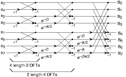
Each term in square brackets has the form of a -length DFT. The first one is a DFT of the even-numbered elements, and the second of the odd-numbered elements. Thefirst DFT is combined with the second multiplied by the complex exponential . The half-length transforms are each evaluated at frequency indices . Normally, the number of frequency indices in a DFT calculation range between zero and the transform length minusone. The computational advantage of the FFT comes from recognizing the periodic nature of the discrete Fouriertransform. The FFT simply reuses the computations made in the half-length transforms and combines them through additions andthe multiplication by , which is not periodic over , to rewrite the length-N DFT. [link] illustrates this decomposition. As it stands, we now compute two length- transforms (complexity ), multiply one of them by the complex exponential (complexity ), and add the results (complexity ). At this point, the total complexity is still dominated by the half-length DFT calculations, but the proportionalitycoefficient has been reduced.
Now for the fun. Because , each of the half-length transforms can be reduced to two quarter-length transforms, each of these to two eighth-lengthones, etc. This decomposition continues until we are left with length-2 transforms. This transform is quite simple, involvingonly additions. Thus, the first stage of the FFT has length-2 transforms (see the bottom part of [link] ). Pairs of these transforms are combined by adding one to the other multiplied by a complexexponential. Each pair requires 4 additions and 4 multiplications, giving a total number of computations equaling . This number of computations does not change from stage to stage. Because the number of stages, the number of times thelength can be divided by two, equals , the complexity of the FFT is .

Notification Switch
Would you like to follow the 'Signals and systems' conversation and receive update notifications?

|
|

|
|

|
|
|
|
|

|
|

|
|

|
|

|
|

|
|

|