<< Chapter < Page Chapter >> Page >

Real time implementation

The environment

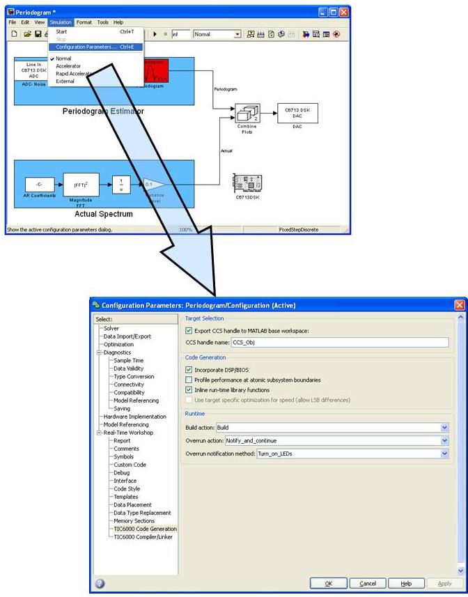
Figure 21 shows the block-diagram for the real time implementation. The DSP will deliver two outputs. The first is the reference spectrum; the second is an estimated spectrum of the output of the all-pole filter. Three real-time models will be created, each one corresponding to an estimator. The user will be able to select the desired estimator through a Graphic User Interface (GUI).

Real Time Implementation Environment

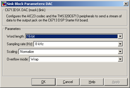
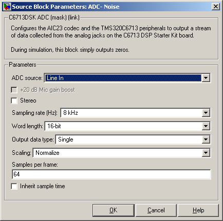
The real-time implementation model will be created from the simulation model, after the following changes:

  • The noise generator block will be replaced by the CODEC of the DSK6713
  • The virtual scope will be replaced also by the CODEC
  • A target definition block (DSK6713) will be added.

Equipment Used:

  • DSK6713
  • Dual Channel Oscilloscope
  • Signal Generator
Real Spectrum Estimation Equipment

Creating the models

  1. Open the simulation model “SpectrumEstimation.mdl”.
  2. Remove the “Burg” and “MCov AR” estimators.
  3. Add the C6713DSK target to the model
    The C6713DSK target Block
  4. Replace the vector scope by the “Digital to Analog” converter (DAC)
    The DAC Block
  5. Configure the DAC block to a sampling rate to 8 KHZ and 16-bit samples.
    The DAC Block Configuration
  6. Double- click on the concatenation object and change the number of inputs from 4 to 2.
  7. Replace the white noise generator by the “Analog to Digital” converter (ADC).
    The ADC Block
  8. Configure the ADC blocks to a sampling rate to 8 KHZ and 16-bit samples.
    The ADC Block Configuration
  9. The final model should look as follows:
    Periodogram Real-Time Model
  10. Set the AR-coefficients data type to single.
  11. Configure the Model to generate and build (without executing) the CCS code as shown:
    Model Configuration
  12. Save the model as “Periodogram.mdl”
  13. Build the model (CTRL-B)
  14. Replace the Periodogram estimator block by the Burg estimator
  15. The final model should look as follows:
    Burg Real-Time Model
  16. Save the model as “Burg.mdl”
  17. Build the model (CTRL-B)
  18. Replace the Burg estimator block by the MCov AR estimator
  19. The final model should look as follows:
    MCov AR Burg Real-Time Model
  20. Save the model as “MCcov_AR.mdl”
  21. Build the model (CTRL-B)At this step you’ll have three .out files to be loaded to the DSK. Each one corresponding to an estimator.

The graphic user interface (gui)

The GUI shown in Figure 32 will be used to select the model. Upon selecting a model, its correspondent load file will be loaded to the DSP.
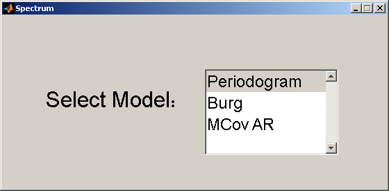
Graphic User Interface (GUI)
  1. Enter GUIDE in the MATLAB® command line.
  2. Choose a new GUI, and name it Spectrum
  3. Add a list-box to your GUI with the string: Periodogram BurgM-Cov
  4. A script file “spectrum.m” will open, when you press the “play” button. Name the script “spectrum.m”
  5. The GUI will perform the following tasks:
    • Upon activating the GUI, the default model is loaded to the DSP.
    • When the user selects a new model, it is loaded to the DSP.
  6. The initialization routine “Spectrum_OpeningFcn” will be: function Spectrum_OpeningFcn(hObject, eventdata, handles, varargin) modelName = gcs;%connect to target: CCS_Obj = connectToCCS(modelName);% Identify RTDX channel names/modes CodegenDir = fullfile(pwd, ['Periodogram' '_c6000_rtw']); OutFile = fullfile(CodegenDir, ['Periodogram' '.out']); %load the model to the DSK:CCS_Obj.load(OutFile,20); handles.CCS_Obj=CCS_Obj;handles.output = hObject; %remember the current model:handles.last_model=1; CCS_Obj.run;% Update handles structure guidata(hObject, handles);
  7. Selecting a new model: %1. halts the current model %2. loads the current model%inputs: %m - 3 levels flag that tells which model to load.%CCS_Obj - the target object function ChangeModel(m,CCS_Obj)CCS_Obj.halt; switch mcase 1 model='Periodogram';case 2 model='Burg';case 3 model= 'MCov_AR';end CodegenDir = fullfile(pwd, [model '_c6000_rtw']); OutFile = fullfile(CodegenDir, [model '.out']); CCS_Obj.load(OutFile,20);CCS_Obj.run; if last_y~=15000r.writemsg(chan_struct(2).name,1/last_y); end
  8. When the user changes the model, the list-box handler function is invoked: function listbox1_Callback(hObject, eventdata, handles) handles.last_model=get(hObject,'Value') ;ChangeModel(handles.last_model,handles.CCS_Obj); guidata(hObject, handles);

The handler saves the new model as the current model and invokes the change model function we described above.

Now you can run the model, and observe the results in the oscilloscope for the various estimators.

Get Jobilize Job Search Mobile App in your pocket Now!

Get it on Google Play Download on the App Store Now


Source:  OpenStax, From matlab and simulink to real-time with ti dsp's. OpenStax CNX. Jun 08, 2009 Download for free at http://cnx.org/content/col10713/1.1
Google Play and the Google Play logo are trademarks of Google Inc.

Notification Switch

Would you like to follow the 'From matlab and simulink to real-time with ti dsp's' conversation and receive update notifications?

Ask