0.1 Principal component analysis (pca)

Principal component analysis

PCA is essentially just SVD. The only difference is that we usually center the data first using some grand mean before doing SVD. There are three perspectives of views for PCA. Each of them gives different insight on what PCA does.

Low-rank approximation

where Frobenius norm is a matrix version of sums of squared. This gives the interpretation of dimension reduction. Solution to the problem is: $Z={\displaystyle \sum _{i=1}^K{U}_k{d}_k{V}_K^T}$

We do lose some information when doing dimension reduction, but the majority of variance is explained in the lower-rank matrix (The eigenvalues give us information about how significant the eigenvector is. So we put the eigenvalues in the order of the magnitude of the eigenvectors, and discard the smallest several since the contribution of components along that particular eigenvector is less significant comparing that with a large eigenvalue). PCA guarantees the best rank-K approximation to X. The tuning parameter K can be either chosen by cross-validation or AIC/BIC. This property is useful for data visualization when the data is high dimensional.

Matrix factorization

This gives the interpretation of pattern recognition. The first column of U gives the first major pattern in sample (row) space while the first column of V gives the first major pattern in feature space. This property is also useful in recommender systems (a lot of the popular algorithms in collaborative filtering like SVD++, bias-SVD etc. are based upon this “projection-to-find-major-pattern” idea).

Covariance

$$X^{T}X$$ here behaves like covariates for multivariate Gaussian. This is essentially an eigenvalue problem of covariance: $$X^{T}X=V{D}^2{V}^T$$ and $$X{X}^T=U{D}^2{U}^T$$ . Interpretation here is that we are maximizing the covariates in column and row space.

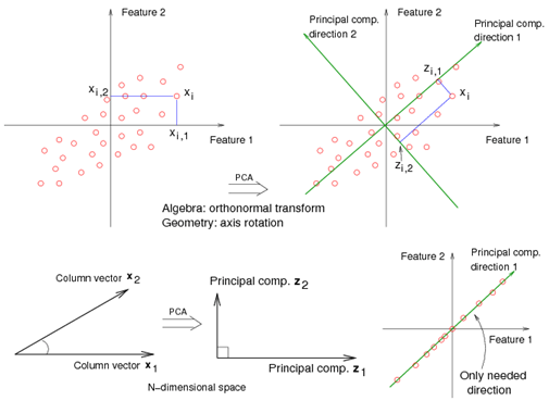
(Figure Credit: https://onlinecourses.science.psu.edu/stat857/node/35)

The intuition behind pca

The intuition behind PCA is as follows: The First PC (Principal Component) finds the linear combinations of variables that correspond to the direction with maximal sample variance (the major pattern of the dataset, the most spread out direction). Succeeding PCs then goes on to find direction that gives highest variance under the constraint of it being orthogonal (uncorrelated) to preceding ones. Geometrically, what we are doing is basically a coordinate transformation – the newly formed axes correspond to the newly constructed linear combination of variables. The number of the newly formed coordinate axes (variables) is usually much lower than the number of axes (variables) in the original dataset, but it’s still explaining most of the variance present in the data.

Another interesting insight

Another interesting insight on PCA is provided by considering its relationship to Ridge Regression (L2 penalty). The result given by Ridge Regression can be written like this:

The term in the middle here, $\frac{d{}_j{}^2}{d_j^2+\lambda }$ , shrinks the singular values. For those major patterns with large singular values, lambda has little effect for shrinking; but for those with small singular values, lambda has huge effect to shrink them towards zero (not exactly zero, unlike lasso - L1 penalty, which does feature selection). This non-uniform shrinkage thus has a grouping effect. This is why Ridge Regression is often used when features are strongly correlated (it only captures orthogonal major pattern). PCA is really easy to implement - feed the data matrix(n*p) to the SVD command in Matlab, extract the PC loading(V) and PC score(U) vector and we will get the major pattern we want.