

| << Chapter < Page | Chapter >> Page > |
We begin by reviewing two notions of convexity: for sets and for functions.
Definition 1 A subset is called convex if for every and ; is called a convex combination of and .
Definition 2 Let be a convex set. A functional is convex on if for all and . If strict inequality holds the functional is set to be strictly convex . A functional is called concave (strictly concave) if is convex (strictly convex).
We will denote the region above the function defined over a convex set as , sometimes called an epigraph , as illustrated in [link] .

Definition 3 Let be a convex functional on a convex set . The conjugate set is defined as
and the conjugate functional is defined as
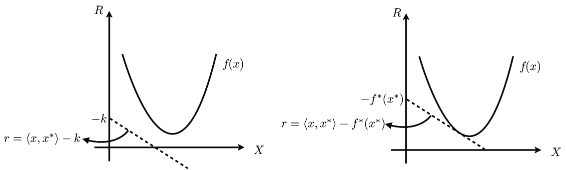
There is a geometric intuition behind the definition of the conjugate functionals. Consider the illustration below where the horizontal axis represents the space and the vertical axis represents the scalar field. A hyperplane in this space contains all points for which for some value of ; the vector determines the orientation of the hyperplane and the value determines the shift from the origin (i.e., the intersect in the axis ). The value of the functional corresponds to the supremum value of for which the hyperplane intersects , and is finite only for ; this is illustrated in [link] .
Note that is convex and is convex. This definition is easily extended to concave functionals.
Definition 4 Let be a concave functional on a convex set . The conjugate set is defined as
and the conjugate functional is defined as
Note that is convex and is concave.
The following theorem will allow us to convert an optimization problem with a convex objective function into a dual problem with a concave objective function.
Theorem 1 (Fenchel) Assume that and are convex and concave functions, respectively, on convex sets and in a normed space . Assume that contains points in the relative interior of and and that either or has a nonempty interior. Suppose further that
is finite. Then,
where the maximum is achieved by some .
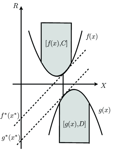
In this theorem, is usually set to zero. From a geometrical point of view, the theorem states that there are two ways to interpret the minimum distance between the two epigraphs and shown below: one in terms of the original functions and one in terms of the duals : we look for the two tangent hyperplanes for and that are maximally separated from one another, as illustrated in [link] .
If the infimum on the left is achieved by , then
Example 1 (Allocation) Assume that we have a capital available for investment with different funds. There is a predicted gain to having stock worth at fund , where the functions are concave. We aim to find the optimal allocation of the capital that maximizes the total gain .
To appeal to duality, we have the concave function and must define a convex function, e.g., . The constraint set can be written as the intersection with
Therefore, we can write our optimization problem as
We consider the conjugate sets. First, we have
We want to define more explicitly. Let be written as , where . Then,
which can be arbitrarily large. Now let ; it is easy to check that for all . If then , which again can be arbitrarily large. Since must hold that , we must have that and so . Since was arbitrary, then .
It is also easy to see that , therefore implying that .
For , we have a conjugate set
since . Now since all vectors in have nonnegative entries. Fix ; if then there is some negative entry among . For such let for some ; then we get which can be arbitrarily close to (i.e., as we have . Thus , a contradiction. Therefore, if then and so . We have therefore shown that .
The conjugate functionals can be written as
since each can be written as . Therefore, can be written as a function of a single variable. Similarly,
where we write
For we can write for all and so
Therefore, the original problem can be reformulated as the following single-variable problem:
This is due to if and only if . Once is found, we can find each as the minimizer in , cf. [link] .
Notification Switch
Would you like to follow the 'Signal theory' conversation and receive update notifications?

|
|

|
|

|
|

|
|

|
|

|
|

|
|

|
|

|
|
|
|