Conditional expectation, regression (Page 3/9)

Applied probability Page 3 / 9

The calculations extend to $E [g (X, Y) | X = t_{i}]$ . Instead of values of u _j we use values of $g (t_{i}, u_{j})$ in the calculations. Suppose $Z = g (X, Y) = Y^{2} - 2 X Y$ .

G = u.^2 - 2*t.*u;         % Z = g(X,Y) = Y^2 - 2XY
EZX = sum(G.*P)./sum(P);   % E[Z|X=x]disp([X;EZX]')0    1.5000
    1.0000    1.50004.0000   -4.0500
    9.0000  -12.8333

Conditioning by a random vector — absolutely continuous case

Suppose the pair ${X, Y}$ has joint density function $f_{X Y}$ . We seek to use the concept of a conditional distribution, given $X = t$ . The fact that $P (X = t) = 0$ for each t requires a modification of the approach adopted in the discrete case. Intuitively, we consider the conditional density

f_{Y | X} (u | t) = \{\begin{matrix} f_{X Y} (t, u) / f_{X} (t) & for f_{X} (t) > 0 \\ 0 & elsewhere \end{matrix})

The condition $f_{X} (t) > 0$ effectively determines the range of X . The function $f_{Y | X} (\cdot | t)$ has the properties of a density for each fixed t for which $f_{X} (t) > 0$ .

f_{Y | X} (u | t) \geq 0, \int f_{Y | X} (u | t) d u = \frac{1}{f_{X} (t)} \int f_{X Y} (t, u) d u = f_{X} (t) / f_{X} (t) = 1

We define, in this case,

E [g (Y) | X = t] = \int g (u) f_{Y | X} (u | t) d u = e (t)

The function $e (\cdot)$ is defined for $f_{X} (t) > 0$ , hence effectively on the range of X . For any reasonable set M on the real line,

E [I_{M} (X) g (Y)] = \int \int I_{M} (t) g (u) f_{X Y} (t, u) d u d t = \int I_{M} (t) [\int g (u) f_{Y | X} (u | t) d u] f_{X} (t) d t

= \int I_{M} (t) e (t) f_{X} (t) d t, where e (t) = E [g (Y) | X = t]

Thus we have, as in the discrete case, for each t in the range of X .

(A) E [I_{M} (X) g (Y)] = E [I_{M} (X) e (X)] where e (t) = E [g (Y) | X = t]

Again, we postpone examination of this pattern until we consider a more general case.

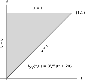
Basic calculation and interpretation

Suppose the pair ${X, Y}$ has joint density $f_{X Y} (t, u) = \frac{6}{5} (t + 2 u)$ on the triangular region bounded by $t = 0$ , $u = 1$ , and $u = t$ (see [link] ). Then

f_{X} (t) = \frac{6}{5} \int_{t}^{1} (t + 2 u) d u = \frac{6}{5} (1 + t - 2 t^{2}), 0 \leq t \leq 1

By definition, then,

f_{Y | X} (u | t) = \frac{t + 2 u}{1 + t - 2 t^{2}} on the triangle (zero elsewhere)

We thus have

E [Y | X = t] = \int u f_{Y | X} (u | t) d u = \frac{1}{1 + t - 2 t^{2}} \int_{t}^{1} (t u + 2 u^{2}) d u = \frac{4 + 3 t - 7 t^{3}}{6 (1 + t - 2 t^{2})} 0 \leq t < 1

Theoretically, we must rule out $t = 1$ since the denominator is zero for that value of t . This causes no problem in practice.

Got questions? Get instant answers now!

Figure one is a cartesian graph in the first quadrant of a labeled, shaded right triangle. The horizontal axis is labeled, t, and the vertical axis is labeled, u. The right triangle appears to have two sides of equal length. Two points, and therefore one side of the triangle sits on the vertical axis, with one point at the origin, and the other further up the graph. This side is labeled, t = 0. The second side of equal length, which begins with one point in the positive region of the vertical axis, and ends in the first quadrant of the graph at the point (1, 1), is labeled u = 1. The hypotenuse of the triangle, which contains one point at the origin and one in the first quadrant of the graph at point (1, 1), is labeled, u = t. There is also a larger caption inside the graph that reads, f_XY (t, u) = (6/5)*(t + 2u). — The density function for [link] .

We are able to make an interpretation quite analogous to that for the discrete case. This also points the way to practical MATLAB calculations.

For any t in the range of X (between 0 and 1 in this case), consider a narrow vertical strip of width $Δ t$ with the vertical line through t at its center. If the strip is narrow enough, then $f_{X Y} (t, u)$ does not vary appreciably with t for any u .
The mass in the strip is approximately
$Mass \approx Δ t \int f_{X Y} (t, u) d u = Δ t f_{X} (t)$
The moment of the mass in the strip about the line $u = 0$ is approximately
$Moment \approx Δ t \int u f_{X Y} (t, u) d u$
The center of mass in the strip is
$Center of mass = \frac{Moment}{Mass} \approx \frac{Δ t \int u f_{X Y} (t, u) d u}{Δ t f_{X} (t)} = \int u f_{Y | X} (u | t) d u = e (t)$

This interpretation points the way to the use of MATLAB in approximating the conditional expectation. The success of the discrete approach in approximating the theoretical valuein turns supports the validity of the interpretation. Also, this points to the general result on regression in the section, "The Regression Problem" .

In the MATLAB handling of joint absolutely continuous random variables, we divide the region into narrow vertical strips. Then we deal with each of these by dividing thevertical strips to form the grid structure. The center of mass of the discrete distribution over one of the t chosen for the approximation must lie close to the actual center of mass of the probability in the strip. Consider the MATLAB treatment of the exampleunder consideration.

<< Chapter < Page Page > Chapter >>

Read also:

Get Jobilize Job Search Mobile App in your pocket Now!

100% Free Mobile Applications
Receive real-time job alerts and never miss the right job again

Source: OpenStax, Applied probability. OpenStax CNX. Aug 31, 2009 Download for free at http://cnx.org/content/col10708/1.6

Google Play and the Google Play logo are trademarks of Google Inc.

Notification Switch

Would you like to follow the 'Applied probability' conversation and receive update notifications?

Ask

	1 Arts Society: Theater 1 By Jonathan Long Start Quiz
	1 Timeshare 1 By Jams Kalo Start Quiz
	13 AP 13 Nervous System MCQ By OpenStax Start Quiz
©flickr:	Microbiology Final By Szilárd Jankó Start Quiz
	Fluid Mechanics MCQ By Stephanie Redfern Start Quiz
	32 Biology 32 Plant Reproduction MCQ By OpenStax Start Quiz
	20 Biology 20 Phylogenies the History of Life MCQ By OpenStax Start Quiz
	1 BOD - DERMATOLOGY - By Brooke Delaney Start Exam
	Introduction to Mechanics MCQ By Saylor Foundation Start Quiz
	2 BOD - Neuropathology By Brooke Delaney Start Exam