0.10 Constrained least squares (cls) problem  (Page 5/5)

It is worth noting that the polynomial weighting form works even when no transition bands are specified (this must become evident from [link] .c above). However, the user must be aware of some practical issues related to this approach. [link] shows a typical CLS polynomial weighting function. Its "spiky" character becomes more dramatic as $p$ increases (the method still follows the homotopy and partial updating ideas from previous sections) as shown in [link] .b. It must be evident that the algorithm will assign heavy weights to frequencies with large errors, but at $p$ increases the difference in weighting exaggerates. At some point the user must make sure that proper sampling is done to ensure that frequencies with large weights (from a theoretical perspective) are being included in the problem, without compromising conputational efficiency (by means of massive oversampling, which can lead to ill-conditioning in numerical least squares methods). Also as $p$ increases, the range of frequencies with signifficantly large weights becomes narrower, thus reducing the overall weighting effect and affecting convergence speed.

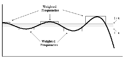
A second weighting form can be defined where envelopes are used. The envelope weighting function approach works by assigning a weight to all frequencies not meeting a constraint. The value of such weights are assigned as flat intervals as illustrated in [link] . Intervals are determined by the edge frequencies within neighborhoods around peak error frequencies for which constraints are not met. Clearly these neighborhoods could change at each iteration. The weight of the $k$ -th interval is still determined by our typical expression,

where ${\omega }_k^{+}$ is the frequency with largest error within the $k$ -th interval.

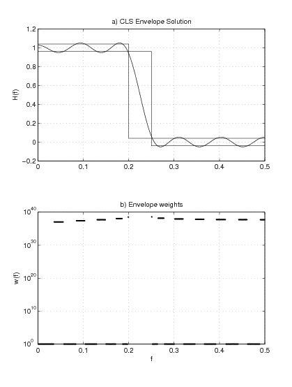
Envelope weighting has been applied in practice with good results. It is particularly effective at reaching high values of $p$ without ill-conditioning, allowing for a true alternative to minimax design. [link] shows an example using $\tau =0.4$ ; the algorithm managed to find a solution for $p=500$ . By specifying transition bands and unachievable constraints one can produce an almost equiripple solution in an efficient manner, with the added flexibility that milder constraints will result in CLS designs.

Comparison with $l_p$ Problem

This chapter presented two problems with similar effects. On one hand, [link] illustrated the fact (see [link] ) that as $p$ increases towards infinity, an $l_p$ filter will approximate an $l_{\infty }$ one. On the other hand, [link] presented the constrained least squared problem, and introduced IRLS-based algorithms that produce filters that approximate equiripple behavior as the constraint specifications tighten.

A natural question arises: how do these methods compare with each other? In principle it should be possible to compare their performances, as long as the necessary assumptions about the problem to be solved are compatible in both methods. [link] shows a comparison of these algorithms with the following specifications:

• Both methods designed length-21 Type-I lowpass linear phase digital filters with fixed transition bands defined by $f=\{0.2,0.24\}$ (in normalized linear frequency).
• The $l_p$ experiment used the following values of $p$ :
  $$p=\{2,2.2,2.5,3,4,5,7,10,15,20,30,50,70,100,170,400\}$$
• The CLS experiment used the polynomial weighting method with fixed transition bands and a value of $p=60$ . The error tolerances were
  $$\tau =\{.06,.077,.078,.8,.084,.088,.093,.1,.11,.12,.13,.14,.15,.16,.17,.18\}$$

Some conclusions can be derived from [link] . Even though at the extremes of the curves they both seem to meet, the CLS curve lies just below the $l_p$ curve for most values of $p$ and $\tau$ . These two facts should be expected: on one hand, in principle the CLS algorithm gives an $l_2$ filter if the constraints are so mild that they are not active for any frequency after the first iteration (hence the two curves should match around $p=2$ ). On the other hand, once the constraints become too harsh, the fixed transition band CLS method basically should design an equiripple filter, as only the active constraint frequencies are $l_p$ -weighted (this effects is more noticeable with higher values of $p$ ). Therefore for tight constraints the CLS filter should approximate an $l_{\infty }$ filter.

The reason why the CLS curve lies under the $l_p$ curve is because for a given error tolerance (which could be interpreted as for a given minimax error ${\epsilon }_{\infty }$ ) the CLS method finds the optimal $l_2$ filter. An $l_p$ filter is optimal in an $l_p$ sense; it is not meant to be optimal in either the $l_2$ or $l_{\infty }$ senses. Hence for a given $\tau$ it cannot beat the CLS filter in an $l_2$ sense (it can only match it, which happens around $p=2$ or $p=\infty$ ).

It is important to note that both curves are not drastically different. While the CLS curve represents optimality in an $l_2-l_{\infty }$ sense, not all the problems mentioned in this work can be solved using CLS filters (for example, the magnitude IIR problem presented in [link] ). Also, one of the objectives of this work is to motivate the use of $l_p$ norms for filter design problems, and the proposed CLS implementations (which absolutely depends on IRLS-based $l_p$ formulations) are good examples of the flexibility and value of $l_p$ IRLS methods discussed in this work.