<< Chapter < Page Chapter >> Page >
n = 0 ( r n ) x n = 1 + r x + r ( r 1 ) 2 ! x 2 + + r ( r 1 ) ( r n + 1 ) n ! x n + .

We now need to determine the interval of convergence for the binomial series [link] . We apply the ratio test. Consequently, we consider

| a n + 1 | | a n | = | r ( r 1 ) ( r 2 ) ( r n ) | x | | n + 1 ( n + 1 ) ! · n | r ( r 1 ) ( r 2 ) ( r n + 1 ) | | x | n = | r n | | x | | n + 1 | .

Since

lim n | a n + 1 | | a n | = | x | < 1

if and only if | x | < 1 , we conclude that the interval of convergence for the binomial series is ( −1 , 1 ) . The behavior at the endpoints depends on r . It can be shown that for r 0 the series converges at both endpoints; for −1 < r < 0 , the series converges at x = 1 and diverges at x = −1 ; and for r < −1 , the series diverges at both endpoints. The binomial series does converge to ( 1 + x ) r in ( −1 , 1 ) for all real numbers r , but proving this fact by showing that the remainder R n ( x ) 0 is difficult.

Definition

For any real number r , the Maclaurin series for f ( x ) = ( 1 + x ) r is the binomial series. It converges to f for | x | < 1 , and we write

( 1 + x ) r = n = 0 ( r n ) x n = 1 + r x + r ( r 1 ) 2 ! x 2 + + r ( r 1 ) ( r n + 1 ) n ! x n +

for | x | < 1 .

We can use this definition to find the binomial series for f ( x ) = 1 + x and use the series to approximate 1.5 .

Finding binomial series

  1. Find the binomial series for f ( x ) = 1 + x .
  2. Use the third-order Maclaurin polynomial p 3 ( x ) to estimate 1.5 . Use Taylor’s theorem to bound the error. Use a graphing utility to compare the graphs of f and p 3 .
  1. Here r = 1 2 . Using the definition for the binomial series, we obtain
    1 + x = 1 + 1 2 x + ( 1 / 2 ) ( 1 / 2 ) 2 ! x 2 + ( 1 / 2 ) ( 1 / 2 ) ( 3 / 2 ) 3 ! x 3 + = 1 + 1 2 x 1 2 ! 1 2 2 x 2 + 1 3 ! 1 · 3 2 3 x 3 + ( −1 ) n + 1 n ! 1 · 3 · 5 ( 2 n 3 ) 2 n x n + = 1 + n = 1 ( −1 ) n + 1 n ! 1 · 3 · 5 ( 2 n 3 ) 2 n x n .
  2. From the result in part a. the third-order Maclaurin polynomial is
    p 3 ( x ) = 1 + 1 2 x 1 8 x 2 + 1 16 x 3 .

    Therefore,
    1.5 = 1 + 0.5 1 + 1 2 ( 0.5 ) 1 8 ( 0.5 ) 2 + 1 16 ( 0.5 ) 3 1.2266.

    From Taylor’s theorem, the error satisfies
    R 3 ( 0.5 ) = f ( 4 ) ( c ) 4 ! ( 0.5 ) 4

    for some c between 0 and 0.5 . Since f ( 4 ) ( x ) = 15 2 4 ( 1 + x ) 7 / 2 , and the maximum value of | f ( 4 ) ( x ) | on the interval ( 0 , 0.5 ) occurs at x = 0 , we have
    | R 3 ( 0.5 ) | 15 4 ! 2 4 ( 0.5 ) 4 0.00244 .

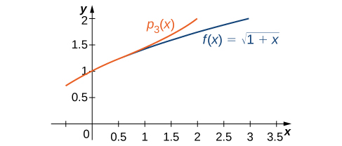
    The function and the Maclaurin polynomial p 3 are graphed in [link] .
    This graph has two curves. The first one is f(x)= the square root of (1+x) and the second is psub3(x). The curves are very close at y = 1.
    The third-order Maclaurin polynomial p 3 ( x ) provides a good approximation for f ( x ) = 1 + x for x near zero.
Got questions? Get instant answers now!

Find the binomial series for f ( x ) = 1 ( 1 + x ) 2 .

n = 0 ( −1 ) n ( n + 1 ) x n

Got questions? Get instant answers now!

Common functions expressed as taylor series

At this point, we have derived Maclaurin series for exponential, trigonometric, and logarithmic functions, as well as functions of the form f ( x ) = ( 1 + x ) r . In [link] , we summarize the results of these series. We remark that the convergence of the Maclaurin series for f ( x ) = ln ( 1 + x ) at the endpoint x = 1 and the Maclaurin series for f ( x ) = tan −1 x at the endpoints x = 1 and x = −1 relies on a more advanced theorem than we present here. (Refer to Abel’s theorem for a discussion of this more technical point.)

Maclaurin series for common functions
Function Maclaurin Series Interval of Convergence
f ( x ) = 1 1 x n = 0 x n −1 < x < 1
f ( x ) = e x n = 0 x n n ! < x <
f ( x ) = sin x n = 0 ( −1 ) n x 2 n + 1 ( 2 n + 1 ) ! < x <
f ( x ) = cos x n = 0 ( −1 ) n x 2 n ( 2 n ) ! < x <
f ( x ) = ln ( 1 + x ) n = 0 ( −1 ) n + 1 x n n −1 < x 1
f ( x ) = tan −1 x n = 0 ( −1 ) n x 2 n + 1 2 n + 1 −1 < x 1
f ( x ) = ( 1 + x ) r n = 0 ( r n ) x n −1 < x < 1

Earlier in the chapter, we showed how you could combine power series to create new power series. Here we use these properties, combined with the Maclaurin series in [link] , to create Maclaurin series for other functions.

Practice Key Terms 2

Get Jobilize Job Search Mobile App in your pocket Now!

Get it on Google Play Download on the App Store Now


Source:  OpenStax, Calculus volume 2. OpenStax CNX. Feb 05, 2016 Download for free at http://cnx.org/content/col11965/1.2
Google Play and the Google Play logo are trademarks of Google Inc.

Notification Switch

Would you like to follow the 'Calculus volume 2' conversation and receive update notifications?

Ask