5.7 Change of variables in multiple integrals  (Page 3/13)

Using the definition, we have

Note that the Jacobian is frequently denoted simply by

Note also that

Hence the notation $J\left(u,v\right)=\frac{\partial \left(x,y\right)}{\partial \left(u,v\right)}$ suggests that we can write the Jacobian determinant with partials of $x$ in the first row and partials of $y$ in the second row.

Change of variables for double integrals

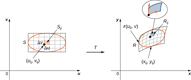
We have already seen that, under the change of variables $T\left(u,v\right)=\left(x,y\right)$ where $x=g\left(u,v\right)$ and $y=h\left(u,v\right),$ a small region $\text{Δ}A$ in the $xy\text{-plane}$ is related to the area formed by the product $\text{Δ}u\text{Δ}v$ in the $uv\text{-plane}$ by the approximation

Now let’s go back to the definition of double integral for a minute:

Referring to [link] , observe that we divided the region $S$ in the $uv\text{-plane}$ into small subrectangles $S_{ij}$ and we let the subrectangles $R_{ij}$ in the $xy\text{-plane}$ be the images of $S_{ij}$ under the transformation $T\left(u,v\right)=\left(x,y\right).$

Then the double integral becomes

Notice this is exactly the double Riemann sum for the integral

With this theorem for double integrals, we can change the variables from $\left(x,y\right)$ to $\left(u,v\right)$ in a double integral simply by replacing

when we use the substitutions $x=g\left(u,v\right)$ and $y=h\left(u,v\right)$ and then change the limits of integration accordingly. This change of variables often makes any computations much simpler.

Changing variables from rectangular to polar coordinates

Consider the integral

${\displaystyle \underset{0}{\overset{2}{\int }}{\displaystyle \underset{0}{\overset{\sqrt{2x-x^2}}{\int }}\sqrt{x^2+y^2}dydx}}.$

Use the change of variables $x=r\text{cos}\theta$ and $y=r\text{sin}\theta ,$ and find the resulting integral.

First we need to find the region of integration. This region is bounded below by $y=0$ and above by $y=\sqrt{2x-x^2}$ (see the following figure).

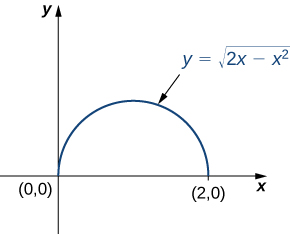
Squaring and collecting terms, we find that the region is the upper half of the circle $x^2+y^2-2x=0,$ that is, $y^2+{\left(x-1\right)}^2=1.$ In polar coordinates, the circle is $r=2\text{cos}\theta$ so the region of integration in polar coordinates is bounded by $0\le r\le \text{cos}\theta$ and $0\le \theta \le \frac{\pi }{2}.$

The Jacobian is $J\left(r,\theta \right)=r,$ as shown in [link] . Since $r\ge 0,$ we have $\left|J\left(r,\theta \right)\right|=r.$

The integrand $\sqrt{x^2+y^2}$ changes to $r$ in polar coordinates, so the double iterated integral is

${\displaystyle \underset{0}{\overset{2}{\int }}{\displaystyle \underset{0}{\overset{\sqrt{2x-x^2}}{\int }}\sqrt{x^2+y^2}}}dydx={\displaystyle \underset{0}{\overset{\pi \text{/}2}{\int }}{\displaystyle \underset{0}{\overset{2\text{cos}\theta }{\int }}r\left|J\left(r,\theta \right)\right|}}drd\theta ={\displaystyle \underset{0}{\overset{\pi \text{/}2}{\int }}{\displaystyle \underset{0}{\overset{2\text{cos}\theta }{\int }}{r}^2}}drd\theta .$

Got questions? Get instant answers now!

Got questions? Get instant answers now!