

| << Chapter < Page | Chapter >> Page > |

Finally, add numeric indicators in a similar fashion as indicated earlier. [link] shows the completed block diagram and front panel.

In this section, let us see how to generate and display aperiodic continuous-time signals or pulses in the time domain. One can represent such signals with a function of time. For simulation purposes, a representation of time is needed. Note that the time scale is continuous while computer programs operate in a discrete fashion. This simulation can be achieved by considering a very small time interval. For example, if a 1-second duration signal in millisecond increments (time interval of 0.001 second) is considered, then one sample every 1 millisecond and a total of 1000 samples are generated for the entire signal. This continuous-time signal approximation is discussed further in later chapters. It is important to note that there is a finite number of samples for a continuous-time signal, and, to differentiate this signal from a discrete-time signal, one must assign a much higher number of samples per second (very small time interval).
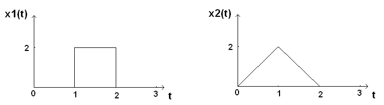
[link] shows two continuous-time signals and with a duration of 3 seconds. By setting the time interval dt to 0.001 second, there is a total of 3000 samples at seconds.
The signal can be represented mathematically as follows:
To simulate this signal, use the LabVIEW MathScript functions
ones and
zeros . The signal value is zero during the first second, which means the first 1000 samples are zero. This portion of the signal is simulated with the function
zeros(1,1000) . In the next second (next 1000 samples), the signal value is 2, and this portion is simulated by the function
2*ones(1,1000) . Finally, the third portion of the signal is simulated by the function
zeros(1,1000) . In other words, the entire duration of the signal is simulated by the following .m file function:
x1=[ zeros(1,1/dt) 2*ones(1,1/dt) zeros(1,1/dt)]
The signal can be represented mathematically as follows:
Use a linearly increasing or decreasing vector to represent the linear portions. The time vectors for the three portions or segments of the signal are
0:dt:1-dt ,
1:dt:2-dt and
2:dt:3-dt . The first segment is a linear function corresponding to a time vector with a slope of 2; the second segment is a linear function corresponding to a time vector with a slope of -2 and an offset of 4; and the third segment is simply a constant vector of zeros. In other words, simulate the entire duration of the signal for any value of dt by the following .m file function:
x2=[2*(0:dt:(1-dt)) -2*(1:dt:(2-dt))+4 zeros(1,1/dt)].
[link] and [link] show the block diagram and front panel of the above signal generation system, respectively. Display the signals using a Waveform Graph (Controls → Express → Waveform Graph) and a Build Waveform function (Function → Programming → Waveform → Build Waveform) . Note that the default data type in MathScript is double precision scalar. So whenever an output possesses any other data type, one needs to right-click on the output and select the Choose Data Type option. In this example, x1 and x2 are double precision one-dimensional arrays that are specified accordingly.
Notification Switch
Would you like to follow the 'An interactive approach to signals and systems laboratory' conversation and receive update notifications?

|
|

|
|

|
|

|
|
|
|
|

|
|
|
|
|
|
|
|

|
|

|