<< Chapter < Page
  Cơ sở tự động học     Page 4 / 4
Chapter >> Page >

s4 + s3 - s - 1 = 0

Bảng Routh :

s4 1 0 -1 0

s3 1 -1 0 0

s2 1 -1 0

s1 0 0

s0 -1

Hệ số ở hàng s0 được tính bằng cách thay 0 ở hàng s1 bằng , rồi tính hệ số của hàng s0 như sau :

ε ( 1 ) 0 ε = 1 size 12{ { {ε \( - 1 \) - 0} over {ε} } = - 1} {}

Cần phương cách này khi có một zero ở cột một. Vì có một lần đổi dấu ở cột một, nên phương trình đặc trưng có một nghiệm có phần thực dương. Do đó, hệ thống không ổn định.

Tiêu chuẩn hurwitz

Tiêu chuẩn ổn định Hurwitz là phương pháp khác để xác định tất cả nghiệm của phương trình đặc trưng có phần thực âm hay không . Tiêu chuẩn này được áp dụng thông qua việc sử dụng các định thức tạo bởi những hệ số của phương trình đặc trưng.

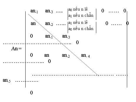
Giả sử hệ số thứ nhất, an dương. Các định thức Ai với i = 1, 2, .... , n-1 được tạo ra như là các định thức con (minor determinant) của định thức :

Các định thức con được lập nên như sau :

Δ 1 = a n 1 Δ 2 = a n 1 a n 3 a n a n 2 = a n 1 a n 2 a n a n 3 Δ 3 = a n 1 a n 3 a n 5 a n a n 2 a n 4 0 a n 1 a n 3 = a n 1 a n 2 a n 3 + a n a n 1 a n 5 a n a n 3 2 a n 4 a n 1 2 alignl { stack { size 12{Δ rSub { size 8{1} } =``a rSub { size 8{n - 1} } } {} #Δ rSub { size 8{2} } = left [ matrix { a rSub { size 8{n - 1} } {} # a rSub { size 8{n - 3} } {} ##a rSub { size 8{n} } {} # a rSub { size 8{n - 2} } {} } right ]`=`a rSub { size 8{n - 1} } a rSub { size 8{n - 2} } ` - ``a rSub { size 8{n} } a rSub { size 8{n - 3} } {} # Δ rSub { size 8{3} } = left [ matrix {a rSub { size 8{n - 1} } {} # a rSub { size 8{n - 3} } {} # a rSub { size 8{n - 5} } {} ## a rSub { size 8{n} } {} # a rSub { size 8{n - 2} } {} # a rSub { size 8{n - 4} } {} ##0 {} # a rSub { size 8{n - 1} } {} # a rSub { size 8{n - 3} } {} } right ]`=a rSub { size 8{n - 1} } a rSub { size 8{n - 2} } `a rSub { size 8{n - 3} } +``a rSub { size 8{n} } a rSub { size 8{n - 1} } a rSub { size 8{n - 5} } {} # ``````````````````````````````````````````````````````````````````` - ``a rSub { size 8{n} } a rSub { size 8{n - 3} } rSup { size 8{2} } ` - a rSub { size 8{n - 4} } a rSub { size 8{n - 1} } rSup { size 8{2} } {}} } {}

Và tăng dần đến ?n

Tất cả các nghiệm của phương trình đặc trưng có phần thực âm nếu và chỉ nếu ?i>0 với i = 1 , 2 , …… , n.

* Thí dụ 6 -10: Với n = 3

Δ 3 = a 2 a 0 0 a 3 a 1 0 0 a 2 a 0 = a 2 a 1 a 0 a 0 2 a 3 size 12{Δ rSub { size 8{3} } ``=`` lline ` matrix { a rSub { size 8{2} } {} # a rSub { size 8{0} } {} # 0 {} ##a rSub { size 8{3} } {} # a rSub { size 8{1} } {} # 0 {} ## 0 {} # a rSub { size 8{2} } {} # a rSub { size 8{0} } {}} ` rline `=``a rSub { size 8{2} } `a rSub { size 8{1} } `a rSub { size 8{0} } ` - `a rSub { size 8{0} } rSup { size 8{2} } `a rSub { size 8{3} } } {}

Δ 2 = a 2 a 0 a 3 a 1 = a 2 a 1 a 0 a 3 size 12{Δ rSub { size 8{2} } `=` lline ` matrix { a rSub { size 8{2} } {} # a rSub { size 8{0} } {} ##a rSub { size 8{3} } {} # a rSub { size 8{1} } {} } rline `=`a rSub { size 8{2} } `a rSub { size 8{1`} } ` - `a rSub { size 8{0} } `a rSub { size 8{3} } } {}

Δ 1 = a 2 size 12{Δ rSub { size 8{1} } `=`a rSub { size 8{2} } } {}

Tất cả các nghiệm của phương trình đặc trưng có phần thực âm nếu

a2>0 , a2 a1 – a0 a3>0

a2 a1 a0 – a02 a3>0

* Thí dụ 6 -11 : Xét sự ổn định của hệ thống có phương trình đặc trưng

s3 + 8s2 + 14s + 24 = 0

Lập các định thức Hurwitz

Δ 3 = 8 24 0 1 14 0 0 8 24 = 88 × 24 > 0 size 12{Δ rSub { size 8{3} } `=` lline ` matrix {8 {} # "24" {} # 0 {} ## 1 {} # "14" {} # 0 {} ##0 {} # 8 {} # "24"{} } ` rline `=``"88"`` times `"24"``>``0} {}

Δ 2 = 8 24 1 14 = 88 > 0 size 12{Δ rSub { size 8{2} } `=` lline ` matrix { 8 {} # "24" {} ##1 {} # "14"{} } ` rline ``=``"88"``>``0} {}

Δ 1 = 8 > 0 size 12{Δ rSub { size 8{1} } `=``8``>``0} {}

Các định thức đều lớn hơn không, các nghiệm của phương trình đặc trưng đều có phần thực âm, nên hệ thống ổn định.

* Thí dụ 6 –12 : Với khoãng giá trị nào của k thì hệ thống sau đây ổn định :

s2 + ks + ( 2k – 1 ) = 0

Δ 2 = k 0 1 2k 1 = k ( 2K 1 ) size 12{Δ rSub { size 8{2} } ``=`` lline ` matrix { k {} # 0 {} ##1 {} # 2k` - `1{} } ` rline ``=``k \( 2K` - `1 \) } {}

Δ 1 = k size 12{Δ rSub { size 8{1} } ``=``k} {}

k (2k -1)>0 k>0

Để hệ ổn định, cần có :

Vậy k > 1 2 size 12{k``>`` { {1} over {2} } } {}

* Thí dụ 6 – 13 :

Một hệ thống thiết kế đạt yêu cầu khi mạch khuếch đại của nó có độ lợi k = 2 . Hãy xác định xem độ lợi này có thể thay đổi bao nhiêu trước khi hệ thống trở nên bất ổn, nếu phương trình đặc trưng của hệ là :

s3+ s2 (4+k) + 6s + 16 + 8k = 0

  • Thay các tham số của phương trình đã cho vào điều kiện Hurwitz tổng quát ở thí dụ 6 –10. Ta được những điều kiện để hệ ổn định :

4 + k>0 , (4+k)6 – (16+8k)>0

(4+k) 6 (16+8k) – (16 + 8k)2>0

Giã sử độ lợi k không thể âm, nên điều kiện thứ nhất thỏa.

Điều kiện thứ nhì và thứ ba thỏa nếu k<4

Vậy với một độ lợi thiết kế có giá trị là 2, hệ thống có thể tăng độ lợi lên gấp đôi trước khi nó trở nên bất ổn.

Độ lợi cũng có thể giãm xuống không mà không gây ra sự mất ổn định.

Bài tập chương vi

VI. 1 Xem nghiệm của phương trình đặc trưng của vài hệ thống điều khiển dưới đây. Hãy xác định trong mỗi trường hợp sự ổn định của hệ. (ổn định, ổn định lề, hay bất ổn)

  1. –1 ,-2 f) 2 , -1 , -3
  2. –1 , +1 g) -6 , -4 , 7
  3. –3 , +2 h) -2 + 3j , -2 – 3j , -2
  4. –1 + j , -1 – j i) -j , j , -1 , 1
  5. –2 +j , -2 – j
  6. 2 , -1 , -3

VI. 2 Môït hệ thống có các cực ở –1 , -5 và các zero ở 1, -2 . Hệ thống ổn định không?

VI. 3 Xét tính ổn định của hệ thống có phương trình đặc trưng :

(s + 1) (s + 2) (s - 3) = 0

VI. 4 Phương trình của một mạch tích phân được viết bởi :

dy/dt = x

Xác định tính ổn định của mạch tích phân.

VI. 5 Tìm đáp ứng xung lực của hệ thống có hàm chuyễn :

G ( s ) = s 2 + 2s + 2 ( s + 1 ) ( s + 2 ) size 12{G \( s \) ``=`` { {s rSup { size 8{2`} } +``2s``+``2} over { \( s+1 \) \( s+2 \) } } } {}

Xét tính ổn định của hệ dựa vào định nghĩa.

VI. 6 Khai triển G(s) thành phân số từng phần. Rồi tìm đáp ứng xung lực và xét tính ổn định.

a) G ( s ) = ( s 2 + s 2 ) s ( s + 1 ) ( s + 2 ) size 12{G \( s \) ``=`` { { - \( s rSup { size 8{2} } +````s``` - ``2 \) } over {s \( s+1 \) \( s+2 \) } } } {}

b) G ( s ) = s 2 + 9 s + 19 s ( s + 1 ) ( s + 2 ) ( s + 4 ) size 12{G \( s \) ``=`` { {s rSup { size 8{2} } +```9`s```+`"19"} over {s \( s+1 \) \( s+2 \) \( s+4 \) } } } {}

VI. 7 Dùng kỹ thuật biến đổi laplace, tìm đáp ứng xung lực của hệ thống diễn tả bởi phương trình vi phân :

d 3 y dt 3 + dy dt = x size 12{ { {d rSup { size 8{3} } y} over { ital "dt" rSup { size 8{3} } } } ``+`` { { ital "dy"} over { ital "dt"} } ```=```x} {} ĐS : y(t) = 1 – cost

VI. 8 Xác định tất cả các cực và zero của :

G ( s ) = s 2 26 s 5 7s 4 30 s 3 size 12{G \( s \) ``=`` { {s rSup { size 8{2`} } ` - "26"} over {s rSup { size 8{5} } - ``7s rSup { size 8{4} } ` - "30"s rSup { size 8{3} } } } } {} ĐS : s3 (s+3)(s-10)

VI. 9 Với mổi đa thức đặc trưng sau đây, xác định tính ổn định của hệ thống.

  1. 2s4 +8s3 + 10s2 + 10s + 20 = 0
  2. s3 + 7s2 + 7s + 46 = 0
  3. s5 + 6s4 + 10s2 + 5s + 24 = 0
  4. s3 - 2s2 + 4s + 6 = 0
  5. s4 +8s3 + 24s2 + 32s + 16 = 0
  6. s6 + 4s4 + 8s2 + 16 = 0 ĐS : b , f : ổn định

VI.10 với giá trị nào của k làm cho hệ thống ổn định, nếu đa thức đặc trưng là :

s3+ (4+k) s2+ 6s + 12 = 0 ĐS : k>2

VI. 11 có bao nhiêu nghiệm có phần thực dương, trong số các đa thức sau đây :

  1. s3 + s2 - s + 1
  2. s4 +2s3 + 2s2 + 2s + 1
  3. s3 + s2 – 2
  4. s4 - s2 - 2s + 2
  5. s3 + s2 + s + 6 ĐS : a(2) , b(0) , c(1) , d(2) , e(2)

VI. 12 Với giá trị dương nào của k làm cho đa thức :

s4 +8s3 + 24s2 + 32s + k = 0

Có các nghiệm với phần thực là zero? Đó là những nghiệm nào?

ĐS : k = 80 , s = ± j2

VI. 13 Hệ thống có phương trình đặc trưung sau đây thì ổnh định?

s4 +3s3 + 6s2 + 9s + 12 = 0

VI. 14 Xác định hàm chuyễn và tìm điều kiện để mạch sau đây ổn định.

ĐS : v 0 ( s ) v i ( s ) = ( s + 1 R 1 C 1 ) ( s + 1 R 2 C 2 ) s 2 + ( 1 R 2 C 2 + 1 R 2 C 1 + 1 R 1 C 1 ) s + 1 R 1 C 1 R 2 C 2 size 12{ { {v rSub { size 8{0} } \( s \) } over {v rSub { size 8{i} } \( s \) } } = { { \( s+ { {1} over {R rSub { size 8{1} } C rSub { size 8{1} } } } \) \( s+ { {1} over {R rSub { size 8{2} } C rSub { size 8{2} } } } \) } over {s rSup { size 8{2} } + \( { {1} over {R rSub { size 8{2} } C rSub { size 8{2} } } } + { {1} over {R rSub { size 8{2} } C rSub { size 8{1} } } } + { {1} over {R rSub { size 8{1} } C rSub { size 8{1} } } } \) s+ { {1} over {R rSub { size 8{1} } C rSub { size 8{1} } R rSub { size 8{2} } C rSub { size 8{2} } } } } } } {}

VI. 15 Xác định hàm chuyễn và tìm điều kiện để mạch sau đây ổn định.

ĐS : v 0 ( s ) v i ( s ) = 1 R 1 R 2 C 1 C 2 s 2 + ( R 1 C 1 + R 1 C 2 + R 2 C 2 ) s + 1 size 12{ { {v rSub { size 8{0} } \( s \) } over {v rSub { size 8{i} } \( s \) } } = { {1} over {R rSub { size 8{1} } R rSub { size 8{2} } C rSub { size 8{1} } C rSub { size 8{2} } s rSup { size 8{2} } + \( R rSub { size 8{1} } C rSub { size 8{1} } +R rSub { size 8{1} } C rSub { size 8{2} } +R rSub { size 8{2} } C rSub { size 8{2} } \) s+1} } } {}

(Dùng bảng Routh)

VI.16 Xác định những điều kiện Hurwith cho sự ổn định của hệ thống có phương trình đặc trưng cấp 4. Giả sử a4>0

a4 s4 + a3 s3 + a2 s2 + a1 s + a0 = 0

ĐS : a3>0 , a3 a2­ – a4 a1­>0 , a3 a2­a1 – a0 a3­2 – a4 a1­2>0

a3 (a2­a1a0 – a3 a0­2 ) – a0 a1­2 a4>0

*****************

Questions & Answers

differentiate between demand and supply giving examples
Lambiv Reply
differentiated between demand and supply using examples
Lambiv
what is labour ?
Lambiv
how will I do?
Venny Reply
how is the graph works?I don't fully understand
Rezat Reply
information
Eliyee
devaluation
Eliyee
t
WARKISA
hi guys good evening to all
Lambiv
multiple choice question
Aster Reply
appreciation
Eliyee
explain perfect market
Lindiwe Reply
In economics, a perfect market refers to a theoretical construct where all participants have perfect information, goods are homogenous, there are no barriers to entry or exit, and prices are determined solely by supply and demand. It's an idealized model used for analysis,
Ezea
What is ceteris paribus?
Shukri Reply
other things being equal
AI-Robot
When MP₁ becomes negative, TP start to decline. Extuples Suppose that the short-run production function of certain cut-flower firm is given by: Q=4KL-0.6K2 - 0.112 • Where is quantity of cut flower produced, I is labour input and K is fixed capital input (K-5). Determine the average product of lab
Kelo
Extuples Suppose that the short-run production function of certain cut-flower firm is given by: Q=4KL-0.6K2 - 0.112 • Where is quantity of cut flower produced, I is labour input and K is fixed capital input (K-5). Determine the average product of labour (APL) and marginal product of labour (MPL)
Kelo
yes,thank you
Shukri
Can I ask you other question?
Shukri
what is monopoly mean?
Habtamu Reply
What is different between quantity demand and demand?
Shukri Reply
Quantity demanded refers to the specific amount of a good or service that consumers are willing and able to purchase at a give price and within a specific time period. Demand, on the other hand, is a broader concept that encompasses the entire relationship between price and quantity demanded
Ezea
ok
Shukri
how do you save a country economic situation when it's falling apart
Lilia Reply
what is the difference between economic growth and development
Fiker Reply
Economic growth as an increase in the production and consumption of goods and services within an economy.but Economic development as a broader concept that encompasses not only economic growth but also social & human well being.
Shukri
production function means
Jabir
What do you think is more important to focus on when considering inequality ?
Abdisa Reply
any question about economics?
Awais Reply
sir...I just want to ask one question... Define the term contract curve? if you are free please help me to find this answer 🙏
Asui
it is a curve that we get after connecting the pareto optimal combinations of two consumers after their mutually beneficial trade offs
Awais
thank you so much 👍 sir
Asui
In economics, the contract curve refers to the set of points in an Edgeworth box diagram where both parties involved in a trade cannot be made better off without making one of them worse off. It represents the Pareto efficient allocations of goods between two individuals or entities, where neither p
Cornelius
In economics, the contract curve refers to the set of points in an Edgeworth box diagram where both parties involved in a trade cannot be made better off without making one of them worse off. It represents the Pareto efficient allocations of goods between two individuals or entities,
Cornelius
Suppose a consumer consuming two commodities X and Y has The following utility function u=X0.4 Y0.6. If the price of the X and Y are 2 and 3 respectively and income Constraint is birr 50. A,Calculate quantities of x and y which maximize utility. B,Calculate value of Lagrange multiplier. C,Calculate quantities of X and Y consumed with a given price. D,alculate optimum level of output .
Feyisa Reply
Answer
Feyisa
c
Jabir
the market for lemon has 10 potential consumers, each having an individual demand curve p=101-10Qi, where p is price in dollar's per cup and Qi is the number of cups demanded per week by the i th consumer.Find the market demand curve using algebra. Draw an individual demand curve and the market dema
Gsbwnw Reply
suppose the production function is given by ( L, K)=L¼K¾.assuming capital is fixed find APL and MPL. consider the following short run production function:Q=6L²-0.4L³ a) find the value of L that maximizes output b)find the value of L that maximizes marginal product
Abdureman
types of unemployment
Yomi Reply
What is the difference between perfect competition and monopolistic competition?
Mohammed
Got questions? Join the online conversation and get instant answers!
Jobilize.com Reply

Get Jobilize Job Search Mobile App in your pocket Now!

Get it on Google Play Download on the App Store Now


Source:  OpenStax, Cơ sở tự động học. OpenStax CNX. Jul 29, 2009 Download for free at http://cnx.org/content/col10756/1.1
Google Play and the Google Play logo are trademarks of Google Inc.

Notification Switch

Would you like to follow the 'Cơ sở tự động học' conversation and receive update notifications?

Ask