2.1 Analysis of time series  (Page 3/6)

If $d<d_L$ , we can reject the null hypothesis of no autocorrelation; if $d_U<d<4-d_U,$ we cannot reject the null hypothesis; and if $d_L<d<d_U,$ the results of the test are uncertain. Moreover, since the distributions are symmetric around 2 and between 0 and 4, the critical values for the alternative hypothesis of negative autocorrelation $(\text{i}\text{. e}\text{.,}$ $\rho >0)$ are 4 minus either the upper or lower critical values, as shown in Figure 3. Critical values for the Durbin-Watson statistic can be found in the appendices of most econometric textbooks.

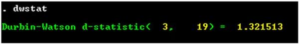
The command for the test and the resultant DW-statistics for the estimate of Equation (2) are shown in Figure 4. The 5 percent level critical values for the Durbin-Watson statistic for a sample size of 19 with two parameters (less the intercept) estimated are 1.074 and 1.536—if the observed value of the DW-statistic is between 1.536 and 2.464, we can accept the null hypothesis that the residuals do not exhibit autocorrelation. Our value of 1.32 falls in the uncertain region where we are not sure if we can or cannot reject the null hypothesis.

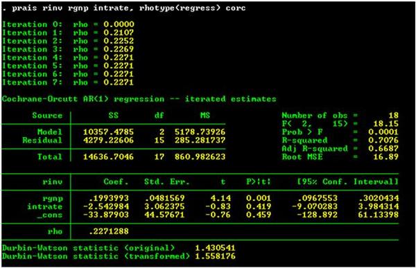
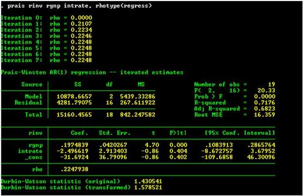
At this point we can try the Cochran-Orcutt estimate. Figure 5 reports the results of using the Cochran-Orcutt estimation procedure. Notice that it took 7 iterations for the estimate of $\rho$ to converge. If we use the Prais-Winsten estimation technique, we get the results shown in Figure 6. It is reassuring to see that the two estimation techniques do not yield estimates of the standard errors that are substantially different from each other.

Using either the Cochran-Orcutt or the Prais-Winstn estimator is dependent on the assumption that the error terms exhibit first-order autocorrelation. Unfortunately, there is no particular reason (from a theoretical viewpoint) to believe in this assumption. Why, for instance, couldn't the error terms of Equation (2) exhibit second-order autocorrelation of the form:

There is a more troubling possible explanation for the low Durbin-Watson statistic: the model may be misspecified . In particular, there may be important explanatory variables omitted from the regression. These omitted explanatory variables may exhibit autocorrelation and, thus, may be the source of autocorrelation in the error term. If the omitted explanatory variables are correlated with the included explanatory variables, then the parameter estimates are biased. The large difference in the estimate of parameter for real interest rates for the OLS regression and the Cochran-Orcutt estimate is suggestive of model misspecification. If the OLS parameter estimates are unbiased but the standard error estimates are, then applying the Cochran-Orcutt adjustment should change the estimates of the standard errors without changing the estimates of the equation parameters substantially.

More modern time-series models

Arma models

The model we described above is assumed to have first-order autoregressive error disturbances. Such a process is referred to as AR(1). The error structure in (8) is AR(2). If we apply this concept to a data series, we would call the following an AR( p ) process: