

| << Chapter < Page | Chapter >> Page > |
In the previous labs, different mathematical transformation tools to represent analog and discrete signals were examined. This final lab builds on the knowledge gained in the previous labs to show how to use these tools to perform signal processing.
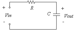
Analog filters are defined over a continuous range of frequencies. Four basic kinds of analog filters are lowpass, highpass, bandpass and bandstop. [link] shows the ideal characteristics of these filters. In the noise removal example of Lab 5 , an ideal lowpass filter was used to remove high-frequency noise. However, the ideal characteristics are not physically realizable and actual filters can only approximate the ideal characteristics. The RC series circuit analyzed in Lab 3 and Lab 4 is a simple example of an analog lowpass filter.

The voltage output for the circuit shown in [link] is given by [link] :
The magnitude and phase response can be easily found to be [link] :
If the positions of R and C are interchanged, a simple analog highpass filter is obtained as shown in [link] .

The voltage output for this circuit is given by
The corresponding magnitude and phase responses are
Digital signal filtering is a fundamental concept in digital signal processing. Two basic kinds of digital filters that are widely used are FIR and IIR:
FIR (finite impulse response) – filters having finite unit sample responses
IIR (infinite impulse response) – filters having infinite unit sample responses
Unit sample response denotes the output in response to a unit input signal. It is common to express digital filters in the form of difference equations. In this form, an FIR filter is expressed as
where ’s denote the filter coefficients andthe filter order. As described by this equation, an FIR filter uses a current input and a number of previous inputs to generate a current output .
The difference equation of an IIR filter is given by
where ’s and ’s denote the filter coefficients and and the number of zeros and poles, respectively. As indicated by Equation (8), an IIR filter uses a number of previous outputs as well as a current and a number of previous inputs to generate a current output .
In general, as compared to IIR filters, FIR filters require less precision and are computationally more stable. Table 1 lists some of the differences between FIR and IIR filters. For the theoretical details on these differences, refer to [link] .
| Attribute | FIR filter | IIR filter |
| Stability | Always stable | Conditionally stable |
| Computational complexity | More operations | Fewer operations |
| Precision | Less coefficient precision required | Higher coefficient precision required |
where ’s and ’s denote the filter coefficients andandthe number of zeros and poles, respectively. As indicated by Equation (8), an IIR filter uses a number of previous outputs as well as a current and a number of previous inputs to generate a current output .
It is well-known that a direct-form implementation expressed by Equation (9) is sensitive, in terms of stability, to coefficient quantization errors. Noting that the second-order cascade form produces a more response that is more resistant to quantization noise [link] , the above transfer function is often written and implemented as follows:
where and represents the largest integer less than or equal to the argument. This serial or cascaded structure is illustrated in [link] .

Each second-order filter is considered to be of direct-form II, shown in [link] , for its memory efficiency. One can implement each second-order filter in software. Normally, digital filters are implemented in software, but one can also implement them in hardware by using digital circuit adders and shifters.

Notification Switch
Would you like to follow the 'An interactive approach to signals and systems laboratory' conversation and receive update notifications?

|
|

|
|

|
|

|
|

|
|

|
|

|
|

|
|

|
|
|
|