<< Chapter < Page Chapter >> Page >
u x x u ( x + d x , t ) - 2 u ( x , t ) + u ( x - d x , t ) d x 2

These approximations may be substituted into our original partial differential equation in order to solve for u ( x , t ) .

The second finite difference method used to solve the wave equation is the trapezoidal approximation method, where we have the system of equations

u u t t = 0 I x x - c ( t ) δ ( x - x c ) u u t + 0 b ( t ) δ ( x - x b )

which we will denote as

V ' ( t ) = A ( t ) V ( t ) + B ( t )

where I represents the identity matrix. The x x operator is a tridiagonal matrix with -2 along the diagonal and ones along the superdiagonal and subdiagonal. The approximating integral equation

( j - 1 ) d t j d t V ' ( t ) d t = ( j - 1 ) d t j d t ( A ( t ) V ( t ) + B ( t ) ) d t

is solved to reveal a solution for u ( j d t ) . The trapezoidal integration method turns out to be the more accurate of the two solution methods, since its error is less than the error of the forward Euler method. Real values for the string's tension, density, and length were used to evaluate the solution for the trapezoidal method, but gave us unintelligible results when used for the forward Euler method. Both methods were used to evaluate the solution using arbitrary values.

Optimization

With all the preliminary work established, we can move on to the optimization problem. We investigated two objective functions for optimization. The first objective function considered was the following

J ( c ( t ) ) = 0 ( u ( x , T ; c ( t ) ) - u 0 ( x , T ) ) 2 d x .

Here a suitable time T is preordained. It is legitimate to do this since damping should not affect the periodic details of the waveform. The u ( x , T ) is solved with the given c ( t ) and fitted to u 0 ( x , T ) = sin ( 4 π x ) . We parameterize

c ( t ) = e - c 1 t - e - c 2 t

which acts at one point on the string with a shape similar to the following.

It is important also that c 1 < c 2 to guarantee the above shape. Our control problem then, is to

min c 1 , c 2 0 ( u ( x , T ; c ( t ) ) - u 0 ( x , T ) ) 2 d x

subject to u ( x , T ; c ( t ) ) solving our wave equation with the same initial and boundary conditions. There is a scaling issue since u ( x , T ) is small (on the order of 10 - 5 ) at times. To correct this we scale our target u 0 so that the two waveforms are comparable before we run the optimization. Normalizing u instead, would be cumbersome since the maximum amplitude depends on time. To expedite the optimizer, we supply the gradient of our objective

J ( c ( t ) ) = ( J ( c ( t ) ) c 1 , J ( c ( t ) ) c 2 ) .

The equations for the partial derivatives are as follows.

J ( c ( t ) ) c 1 = 2 0 ( u ( x , T ; c ( t ) ) - u 0 ( x , T ) ) ( u ( x , T , c ( t ) ) c 1 ) d x ,
J ( c ( t ) ) c 2 = 2 0 ( u ( x , T ; c ( t ) ) - u 0 ( x , T ) ) ( u ( x , T , c ( t ) ) c 2 ) d x

The inner partial derivatives will be approximated by the same finite difference method we used above.

One of the main difficulties with this objective function is that it requires a T to be found beforehand and thus we can only optimize with respect to our spacial dimension. Optimizing over both space and time would rid us of needing to find a good T but complicates our objective function and retards our optimizer. Another concern with this objective is that it takes into account the sign of the target waveform, but whether the waveform is sin ( x ) or - sin ( x ) is no matter to the musician. Along the same lines we have the scaling difficulty. Another objective function we have explored is the following energy minimization problem. We note that u ( x , t ) can be represented as a combination of sinusoids. For a given T we have

u ( x , T ) = n = 1 N u n sin ( 2 n π x ) .

Here each u n represents the nth Fourier coefficient that corresponds to the expression of the nth mode in the total wave. Since we are interested in expressing only the fourth mode, our optimization problem will try to minimize all other modes

min c 1 , c 2 F ( c ( t ) ) = 0 T f i n n = 1 , n 4 10 0 ( u ( x , t ; c ( t ) ) sin n π x d x 2 d t

subject to our wave equation with the same conditions. We decide on clearing up the first ten modes (except the fourth) to ensure that we are left with a waveform closest to our target. Like before we supply the gradient.

F ( c ( t ) ) c 1 = 2 0 T f i n n = 1 , n 4 10 0 ( u ( x , t ; c ( t ) ) sin n π x u ( x , t , c ( t ) ) c 1 d x d t ,
F ( c ( t ) ) c 2 = 2 0 T f i n n = 1 , n 4 10 0 ( u ( x , t ; c ( t ) ) sin n π x u ( x , t , c ( t ) ) c 2 d x d t .

This objective function solves the sign and amplitude problems of the first. Additionally we are now optimizing over time so we need not specify a T . One may wish to reset the bounds of the time integral through a different interval.

Results

This is the result of our optimizer given a certain driving force b ( t ) using our first objective function.

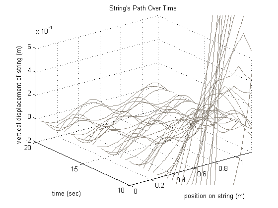
This is the result of our optimizer at a certain time using the energy minimization objective. Since we optimized over space and time, we express this as a three dimensional plot.

For the energy minimization objective function using multiple dampings, we have this result.

Comparatively, the values of the objective function for single and multiple dampings are on the same order of magnitude, with the value for the single dampings being slightly smaller. Therefore the optimization process for a single damping is more effective, but not by much.

Acknowledgments

We would like to give a big thanks to Dr. Steve Cox for his guidance and support throughout the course of the project. This paper describes work completed with the support of the NSF.

Appendix

All of the codes used in this project are available on our website at

http://www.owlnet.rice.edu/ mlg6/strings/.

References

  1. Bamerger, A., J. Rauch and M. Taylor. A model for harmonics on stringed instruments . Arch. Rational Mech. Anal. 79(1982) 267-290.
  2. Cheney, E. W., and David Kincaid. Numerical Mathematics and Computing . Pacific Grove, CA: Brooks/Cole Pub., 1994. Print.
  3. Cox, S., and Antoine Hernot. Eliciting Harmonics on Strings . ESAIM: COCV 14(2008) 657-677.
  4. Fletcher, Neville H., and Thomas D. Rossing. The Physics of Musical Instruments . New York: Springer-Verlag, 1991. Print.
  5. Knobel, Roger. An Introduction to the Mathematical Theory of Waves . Providence, RI: American Mathematical Society, 2000. Print.
  6. Rayleigh, John William Strutt, and Robert Bruce Lindsay. The Theory of Sound . New York: Dover, 1945. Print.

Questions & Answers

how does the planets on our solar system orbit
cheten Reply
how many Messier objects are there in space
satish Reply
did you g8ve certificate
Richard Reply
what are astronomy
Issan Reply
Astronomy (from Ancient Greek ἀστρονομία (astronomía) 'science that studies the laws of the stars') is a natural science that studies celestial objects and phenomena. It uses mathematics, physics, and chemistry in order to explain their origin and evolution.
Rafael
vjuvu
Elgoog
what is big bang theory?
Rosemary
what type of activity astronomer do?
Rosemary
No
Richard
the big bang theory is a theory which states that all matter was compressed together in one place the matter got so unstable it exploded releasing All its contents in the form of hydrogen
Roaul
I want to be an astronomer. That's my dream
Astrit
Who named the the whole galaxy?
Shola Reply
solar Univers
GPOWER
what is space
Richard
what is the dark matter
Richard
what are the factors upon which the atmosphere is stratified
Nicholas Reply
is the big bang the sun
Folakemi Reply
no
Sokak
bigbang is the beginning of the universe
Sokak
but thats just a theory
Sokak
nothing will happen, don't worry brother.
Vansh
what does comet means
GANGAIN Reply
these are Rocky substances between mars and jupiter
GANGAIN
Comets are cosmic snowballs of frozen gases , rock and dust that orbit the sun. They are mostly found between the orbits of Venus and Mercury.
Aarya
hllo
John
hi
John
qt rrt
John
r u there
John
hey can anyone guide me abt international astronomy olympiad
sahil
how can we learn right and true ?
Govinda Reply
why the moon is always appear in an elliptical shape
Gatjuol Reply
Because when astroid hit the Earth then a piece of elliptical shape of the earth was separated which is now called moon.
Hemen
what's see level?
lidiya Reply
Did you mean eye sight or sea level
Minal
oh sorry it's sea level
lidiya
according to the theory of astronomers why the moon is always appear in an elliptical orbit?
Gatjuol
hi !!! I am new in astronomy.... I have so many questions in mind .... all of scientists of the word they just give opinion only. but they never think true or false ... i respect all of them... I believes whole universe depending on true ...থিউরি
Govinda
hello
Jackson
hi
Elyana
we're all stars and galaxies a part of sun. how can science prove thx with respect old ancient times picture or books..or anything with respect to present time .but we r a part of that universe
w astronomy and cosmology!
Michele
another theory of universe except big ban
Albash Reply
how was universe born
Asmit Reply
there many theory to born universe but what is the reality of big bang theory to born universe
Asmit
what is the exact value of π?
Nagalakshmi
by big bang
universal
there are many theories regarding this it's on you believe any theory that you think is true ex. eternal inflation theory, oscillation model theory, multiple universe theory the big bang theory etc.
Aarya
I think after Big Bang!
Michele
from where on earth could u observe all the stars during the during the course of an year
Karuna Reply
I think it couldn't possible on earth
Nagalakshmi
in this time i don't Know
Michele
is that so. the question was in the end of this chapter
Karuna
in theory, you could see them all from the equator (though over the course of a year, not at pne time). stars are measured in "declination", which is how far N or S of the equator (90* to -90*). Polaris is the North star, and is ALMOST 90* (+89*). So it would just barely creep over the horizon.
Christopher
Got questions? Join the online conversation and get instant answers!
Jobilize.com Reply

Get Jobilize Job Search Mobile App in your pocket Now!

Get it on Google Play Download on the App Store Now


Source:  OpenStax, The art of the pfug. OpenStax CNX. Jun 05, 2013 Download for free at http://cnx.org/content/col10523/1.34
Google Play and the Google Play logo are trademarks of Google Inc.

Notification Switch

Would you like to follow the 'The art of the pfug' conversation and receive update notifications?

Ask