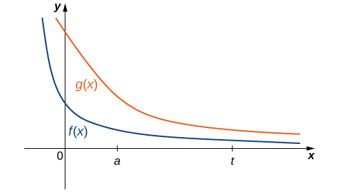
It is not always easy or even possible to evaluate an improper integral directly; however, by comparing it with another carefully chosen integral, it may be possible to determine its convergence or divergence. To see this, consider two continuous functions
and
satisfying
for
(
[link] ). In this case, we may view integrals of these functions over intervals of the form
as areas, so we have the relationship
If
for
then for
Thus, if
then
as well. That is, if the area of the region between the graph of
and the
x -axis over
is infinite, then the area of the region between the graph of
and the
x -axis over
is infinite too.
On the other hand, if
for some real number
then
must converge to some value less than or equal to
since
increases as
increases and
for all
If the area of the region between the graph of
and the
x -axis over
is finite, then the area of the region between the graph of
and the
x -axis over
is also finite.
These conclusions are summarized in the following theorem.
A comparison theorem
Let
and
be continuous over
Assume that
for
If
then
If
where
is a real number, then
for some real number
Applying the comparison theorem
Use a comparison to show that
converges.
We can see that
so if
converges, then so does
To evaluate
first rewrite it as a limit:
In the last few chapters, we have looked at several ways to use integration for solving real-world problems. For this next project, we are going to explore a more advanced application of integration: integral transforms. Specifically, we describe the
Laplace transform and some of its properties. The Laplace transform is used in engineering and physics to simplify the computations needed to solve some problems. It takes functions expressed in terms of time and
transforms them to functions expressed in terms of frequency. It turns out that, in many cases, the computations needed to solve problems in the frequency domain are much simpler than those required in the time domain.
The Laplace transform is defined in terms of an integral as
Note that the input to a Laplace transform is a function of time,
and the output is a function of frequency,
Although many real-world examples require the use of complex numbers (involving the imaginary number
in this project we limit ourselves to functions of real numbers.
Let’s start with a simple example. Here we calculate the Laplace transform of
. We have
This is an improper integral, so we express it in terms of a limit, which gives
Now we use integration by parts to evaluate the integral. Note that we are integrating with respect to
t , so we treat the variable
s as a constant. We have
Then we obtain
Calculate the Laplace transform of
Calculate the Laplace transform of
Calculate the Laplace transform of
(Note, you will have to integrate by parts twice.)
Laplace transforms are often used to solve differential equations. Differential equations are not covered in detail until later in this book; but, for now, let’s look at the relationship between the Laplace transform of a function and the Laplace transform of its derivative.
Let’s start with the definition of the Laplace transform. We have
Use integration by parts to evaluate
(Let
and
After integrating by parts and evaluating the limit, you should see that
Then,
Thus, differentiation in the time domain simplifies to multiplication by
s in the frequency domain.
The final thing we look at in this project is how the Laplace transforms of
and its antiderivative are related. Let
Then,
Use integration by parts to evaluate
(Let
and
Note, by the way, that we have defined
As you might expect, you should see that
Integration in the time domain simplifies to division by
s in the frequency domain.