2.3 Module 4: instruction set: characteristics and functions  (Page 7/7)

The procedure mechanism involves two basic instructions: a call instruction that branches from the present location to the procedure, and a return instruction that returns from the procedure to the place from which it was called. Both of these are forms of branching instructions.

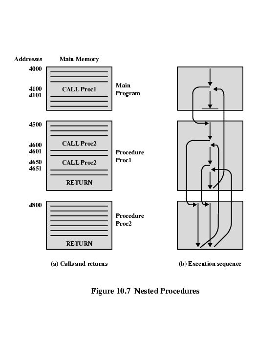
The above figure illustrates the use of procedures to construct a program. In this example, there is a main program starting at location 4000. This program includes a call to procedure PROC1, starting at location 4500. When this call instruction is encountered, the CPU suspends execution of the main program and begins ex­ecution of PROC1 by fetching the next instruction from location 4500. Within PROC1, there are two calls to PR0C2 at location 4800. In each case, the execution of PROC1 is suspended and PROC2 is executed. The RETURN statement causes the CPU to go back to the calling program and continue execution at the instruc­tion after the corresponding CALL instruction. This behavior is illustrated in the right of this figure.

Several points are worth noting:

1. A procedure can be called from more than one location.

2. A procedure call can appear in a procedure. This allows the nesting of proce­dures to an arbitrary depth.

3. Each procedure call is matched by a return in the called program.

Because we would like to be able to call a procedure from a variety of points, the CPU must somehow save the return address so that the return can take place appropriately. There are three common places for storing the return address:

• Register

• Start of called procedure

• Top of stack

4. addressing modes

The address field or fields in a typical instruction format are relatively small. We would like to be able to reference a large range of locations in main memory or for some systems, virtual memory. To achieve this objective, a variety of addressing techniques has been employed. They all involve some trade-off between address range and/or addressing flexibility, on the one hand, and the number of memory ref­erences and/or the complexity of address calculation, on the other. In this section, we examine the most common addressing techniques:

• Immediate
• Direct
• Indirect
• Register
• Register indirect
• Displacement

4.1 immediate addressing

The simplest form of addressing is immediate addressing, in which the operand is actually present in the instruction:

• Operand is part of instruction
• Operand = address field
• e.g. ADD 5 ;Add 5 to contents of accumulator ;5 is operand

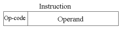
The advantage of immediate addressing is that no memory reference other than the instruction fetch is required to obtain the operand, thus saving one mem­ory or cache cycle in the instruction cycle.

The disadvantage is that the size of the number is restricted to the size of the address field, which, in most instruction sets, is small compared with the word length.

4.2 direct addressing

A very simple form of addressing is direct addressing, in which:

• Address field contains address of operand
• Effective address (EA) = address field (A)
• e.g. ADD A ;Add contents of cell A to accumulator

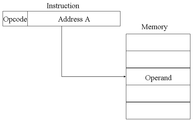
The technique was common in earlier generations of computers but is not common on contemporary architectures. It requires only one memory reference and no spe­cial calculation. The obvious limitation is that it provides only a limited address space.

4.3 indirect addressing

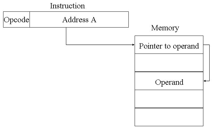
With direct addressing, the length of the address field is usually less than the word length, thus limiting the address range. One solution is to have the address field refer to the address of a word in memory, which in turn contains a full-length address of the operand. This is known as indirect addressing.

4.4 register addressing

Register addressing is similar to direct addressing. The only difference is that the address field refers to a register rather than a main memory address.

The advantages of register addressing are that :

• Only a small address field is needed in the instruction
• No memory 'references are required, faster instruction fetch

The disadvantage of register addressing is that the address space is very limited.

4.5 register indirect addressing

Just as register addressing is analogous to direct addressing, register indirect ad­dressing is analogous to indirect addressing. In both cases, the only difference is whether the address field refers to a memory location or a register. Thus, for register indirect address: Operand is in memory cell pointed to by contents of register.

The advantages and limitations of register indirect addressing are basically the same as for indirect addressing. In both cases, the address space limitation (limited range of addresses) of the address field is overcome by having that field refer to a word-length location containing an address. In addition, register indirect addressing uses one less memory reference than indirect addressing.

4.6 displacement addressing

A very powerful mode of addressing combines the capabilities of direct addressing and register indirect addressing. It is known by a variety of names depending on the context of its use but the basic mechanism is the same. We will refer to this as displacement addressing, address field hold two values:

• A = base value
• R = register that holds displacement