<< Chapter < Page Chapter >> Page >

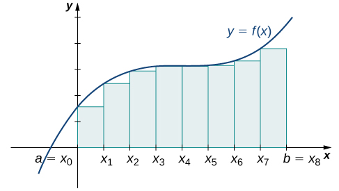
[link] shows the same curve divided into eight subintervals. Comparing the graph with four rectangles in [link] with this graph with eight rectangles, we can see there appears to be less white space under the curve when n = 8 . This white space is area under the curve we are unable to include using our approximation. The area of the rectangles is

L 8 = f ( 0 ) ( 0.25 ) + f ( 0.25 ) ( 0.25 ) + f ( 0.5 ) ( 0.25 ) + f ( 0.75 ) ( 0.25 ) + f ( 1 ) ( 0.25 ) + f ( 1.25 ) ( 0.25 ) + f ( 1.5 ) ( 0.25 ) + f ( 1.75 ) ( 0.25 ) = 7.75.
A graph showing the left-endpoint approximation for the area under the given curve from a=x0 to b = x8. The heights of the rectangles are determined by the values of the function at the left endpoints.
The region under the curve is divided into n = 8 rectangular areas of equal width for a left-endpoint approximation.

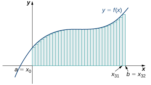
The graph in [link] shows the same function with 32 rectangles inscribed under the curve. There appears to be little white space left. The area occupied by the rectangles is

L 32 = f ( 0 ) ( 0.0625 ) + f ( 0.0625 ) ( 0.0625 ) + f ( 0.125 ) ( 0.0625 ) + + f ( 1.9375 ) ( 0.0625 ) = 7.9375.
A graph of the left-endpoint approximation of the area under the given curve from a = x0 to b = x32. The heights of the rectangles are determined by the values of the function at the left endpoints.
Here, 32 rectangles are inscribed under the curve for a left-endpoint approximation.

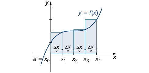
We can carry out a similar process for the right-endpoint approximation method. A right-endpoint approximation of the same curve, using four rectangles ( [link] ), yields an area

R 4 = f ( 0.5 ) ( 0.5 ) + f ( 1 ) ( 0.5 ) + f ( 1.5 ) ( 0.5 ) + f ( 2 ) ( 0.5 ) = 8.5.
A graph of the right-endpoint approximation for the area under the given curve from x0 to x4. The heights of the rectangles are determined by the values of the function at the right endpoints.
Now we divide the area under the curve into four equal subintervals for a right-endpoint approximation.

Dividing the region over the interval [ 0 , 2 ] into eight rectangles results in Δ x = 2 0 8 = 0.25 . The graph is shown in [link] . The area is

R 8 = f ( 0.25 ) ( 0.25 ) + f ( 0.5 ) ( 0.25 ) + f ( 0.75 ) ( 0.25 ) + f ( 1 ) ( 0.25 ) + f ( 1.25 ) ( 0.25 ) + f ( 1.5 ) ( 0.25 ) + f ( 1.75 ) ( 0.25 ) + f ( 2 ) ( 0.25 ) = 8.25.
A graph of the right-endpoint approximation for the area under the given curve from a=x0 to b=x8.The heights of the rectangles are determined by the values of the function at the right endpoints.
Here we use right-endpoint approximation for a region divided into eight equal subintervals.

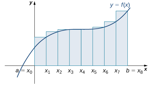
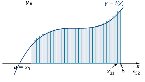
Last, the right-endpoint approximation with n = 32 is close to the actual area ( [link] ). The area is approximately

R 32 = f ( 0.0625 ) ( 0.0625 ) + f ( 0.125 ) ( 0.0625 ) + f ( 0.1875 ) ( 0.0625 ) + + f ( 2 ) ( 0.0625 ) = 8.0625.
A graph of the right-endpoint approximation for the area under the given curve from a=x0 to b=x32. The heights of the rectangles are determined by the values of the function at the right endpoints.
The region is divided into 32 equal subintervals for a right-endpoint approximation.

Based on these figures and calculations, it appears we are on the right track; the rectangles appear to approximate the area under the curve better as n gets larger. Furthermore, as n increases, both the left-endpoint and right-endpoint approximations appear to approach an area of 8 square units. [link] shows a numerical comparison of the left- and right-endpoint methods. The idea that the approximations of the area under the curve get better and better as n gets larger and larger is very important, and we now explore this idea in more detail.

Converging values of left- and right-endpoint approximations as n Increases
Values of n Approximate Area L n Approximate Area R n
n = 4 7.5 8.5
n = 8 7.75 8.25
n = 32 7.94 8.06

Forming riemann sums

So far we have been using rectangles to approximate the area under a curve. The heights of these rectangles have been determined by evaluating the function at either the right or left endpoints of the subinterval [ x i 1 , x i ] . In reality, there is no reason to restrict evaluation of the function to one of these two points only. We could evaluate the function at any point c i in the subinterval [ x i 1 , x i ] , and use f ( x i * ) as the height of our rectangle. This gives us an estimate for the area of the form

Practice Key Terms 8

Get Jobilize Job Search Mobile App in your pocket Now!

Get it on Google Play Download on the App Store Now


Source:  OpenStax, Calculus volume 1. OpenStax CNX. Feb 05, 2016 Download for free at http://cnx.org/content/col11964/1.2
Google Play and the Google Play logo are trademarks of Google Inc.

Notification Switch

Would you like to follow the 'Calculus volume 1' conversation and receive update notifications?

Ask