6.6 Moments and centers of mass  (Page 5/14)

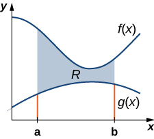
We can adapt this approach to find centroids of more complex regions as well. Suppose our region is bounded above by the graph of a continuous function $f(x),$ as before, but now, instead of having the lower bound for the region be the x -axis, suppose the region is bounded below by the graph of a second continuous function, $g(x),$ as shown in the following figure.

Again, we partition the interval $\left[a,b\right]$ and construct rectangles. A representative rectangle is shown in the following figure.

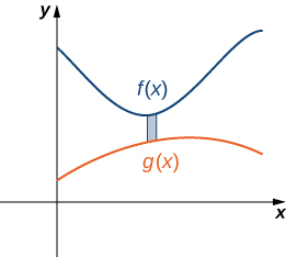
Note that the centroid of this rectangle is $\left(x_i^{*},\left(f(x_i^{*})+g(x_i^{*})\right)\text{/}2\right).$ We won’t go through all the details of the Riemann sum development, but let’s look at some of the key steps. In the development of the formulas for the mass of the lamina and the moment with respect to the y -axis, the height of each rectangle is given by $f(x_i^{*})-g(x_i^{*}),$ which leads to the expression $f(x)-g(x)$ in the integrands.

In the development of the formula for the moment with respect to the x -axis, the moment of each rectangle is found by multiplying the area of the rectangle, $\rho \left[f(x_i^{*})-g(x_i^{*})\right]\text{Δ}x,$ by the distance of the centroid from the x -axis, $\left(f(x_i^{*})+g(x_i^{*})\right)\text{/}2,$ which gives $\rho \left(1\text{/}2\right)\left\{{\left[f(x_i^{*})\right]}^2-{\left[g(x_i^{*})\right]}^2\right\}\text{Δ}x.$ Summarizing these findings, we arrive at the following theorem.

We illustrate this theorem in the following example.

Finding the centroid of a region bounded by two functions

Let R be the region bounded above by the graph of the function $f(x)=1-x^2$ and below by the graph of the function $g(x)=x-1.$ Find the centroid of the region.

The region is depicted in the following figure.

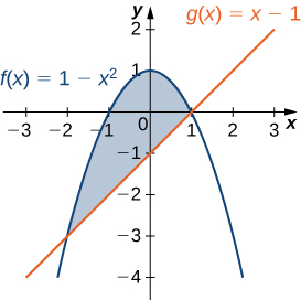
The graphs of the functions intersect at $\left(\mathrm{-2},\mathrm{-3}\right)$ and $(1,0),$ so we integrate from −2 to 1. Once again, for the sake of convenience, assume $\rho =1.$

First, we need to calculate the total mass:

$\begin{array}{cc}\hfill m& =\rho {{\displaystyle \int }}_a^b\left[f(x)-g(x)\right]dx\hfill \\ & ={\displaystyle {\int }_{\mathrm{-2}}^1\left[1-x^2-(x-1)\right]}dx={{\displaystyle \int }}_{\mathrm{-2}}^1(2-x^2-x)dx\hfill \\ & ={\left[2x-\frac{1}{3}{x}^3-\frac{1}{2}{x}^2\right]|}_{\mathrm{-2}}^1=\left[2-\frac{1}{3}-\frac{1}{2}\right]-\left[\mathrm{-4}+\frac{8}{3}-2\right]=\frac{9}{2}.\hfill \end{array}$

Next, we compute the moments:

$\begin{array}{cc}\hfill M_x& =\rho {\displaystyle {\int }_a^b\frac{1}{2}\left({\left[f(x)\right]}^2-{\left[g(x)\right]}^2\right)}dx\hfill \\ & =\frac{1}{2}{\displaystyle {\int }_{\mathrm{-2}}^1\left({\left(1-x^2\right)}^2-{\left(x-1\right)}^2\right)dx}=\frac{1}{2}{{\displaystyle \int }}_{\mathrm{-2}}^1\left(x^4-3x^2+2x\right)dx\hfill \\ & =\frac{1}{2}{\left[\frac{x^5}{5}-x^3+x^2\right]|}_{\mathrm{-2}}^1=-\frac{27}{10}\hfill \end{array}$

and

$\begin{array}{cc}\hfill M_y& =\rho {\displaystyle {\int }_a^{b}x\left[f(x)-g(x)\right]dx}\hfill \\ & ={{\displaystyle \int }}_{\mathrm{-2}}^{1}x\left[(1-x^2)-(x-1)\right]dx={{\displaystyle \int }}_{\mathrm{-2}}^{1}x\left[2-x^2-x\right]dx={{\displaystyle \int }}_{\mathrm{-2}}^1\left(2x-x^4-x^2\right)dx\hfill \\ & ={\left[x^2-\frac{x^5}{5}-\frac{x^3}{3}\right]|}_{\mathrm{-2}}^1=-\frac{9}{4}.\hfill \end{array}$

Therefore, we have

$\bar{x}=\frac{M_y}{m}=-\frac{9}{4}·\frac{2}{9}=-\frac{1}{2}\text{and}\bar{y}=\frac{M_x}{y}=-\frac{27}{10}·\frac{2}{9}=-\frac{3}{5}.$

The centroid of the region is $\left(\text{−}\left(1\text{/}2\right),\text{−}\left(3\text{/}5\right)\right).$

Got questions? Get instant answers now!

Got questions? Get instant answers now!