

| << Chapter < Page | Chapter >> Page > |
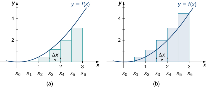
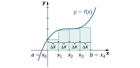
In [link] (b), we draw vertical lines perpendicular to such that is the right endpoint of each subinterval, and calculate for We multiply each by Δ x to find the rectangular areas, and then add them. This is a right-endpoint approximation of the area under Thus,
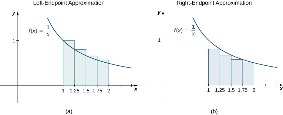
Use both left-endpoint and right-endpoint approximations to approximate the area under the curve of on the interval use
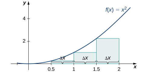
First, divide the interval into n equal subintervals. Using This is the width of each rectangle. The intervals are shown in [link] . Using a left-endpoint approximation, the heights are Then,
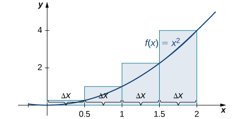
The right-endpoint approximation is shown in [link] . The intervals are the same, but now use the right endpoint to calculate the height of the rectangles. We have
The left-endpoint approximation is 1.75; the right-endpoint approximation is 3.75.
Sketch left-endpoint and right-endpoint approximations for on use Approximate the area using both methods.
The left-endpoint approximation is 0.7595. The right-endpoint approximation is 0.6345. See the below
[link] .
Looking at [link] and the graphs in [link] , we can see that when we use a small number of intervals, neither the left-endpoint approximation nor the right-endpoint approximation is a particularly accurate estimate of the area under the curve. However, it seems logical that if we increase the number of points in our partition, our estimate of A will improve. We will have more rectangles, but each rectangle will be thinner, so we will be able to fit the rectangles to the curve more precisely.
We can demonstrate the improved approximation obtained through smaller intervals with an example. Let’s explore the idea of increasing n , first in a left-endpoint approximation with four rectangles, then eight rectangles, and finally 32 rectangles. Then, let’s do the same thing in a right-endpoint approximation, using the same sets of intervals, of the same curved region. [link] shows the area of the region under the curve on the interval using a left-endpoint approximation where The width of each rectangle is
The area is approximated by the summed areas of the rectangles, or
Notification Switch
Would you like to follow the 'Calculus volume 1' conversation and receive update notifications?

|
|

|
|

|
|

|
|

|
|

|
|

|
|

|
|

|
|

|