| << Chapter < Page | Chapter >> Page > |
Now let’s use this strategy to graph several different functions. We start by graphing a polynomial function.
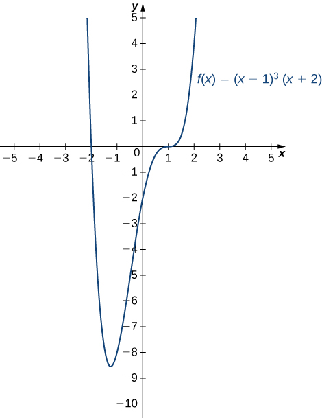
Sketch a graph of
Step 1: Since is a polynomial, the domain is the set of all real numbers.
Step 2: When Therefore, the -intercept is To find the -intercepts, we need to solve the equation gives us the -intercepts and
Step 3: We need to evaluate the end behavior of As and Therefore, As and Therefore, To get even more information about the end behavior of we can multiply the factors of When doing so, we see that
Since the leading term of is we conclude that behaves like as
Step 4: Since is a polynomial function, it does not have any vertical asymptotes.
Step 5: The first derivative of is
Therefore, has two critical points: Divide the interval into the three smaller intervals: and Then, choose test points and from these intervals and evaluate the sign of at each of these test points, as shown in the following table.
| Interval | Test Point | Sign of Derivative | Conclusion |
|---|---|---|---|
| is increasing. | |||
| is decreasing. | |||
| is increasing. |
From the table, we see that has a local maximum at and a local minimum at Evaluating at those two points, we find that the local maximum value is and the local minimum value is
Step 6: The second derivative of is
The second derivative is zero at Therefore, to determine the concavity of divide the interval into the smaller intervals and and choose test points and to determine the concavity of on each of these smaller intervals as shown in the following table.
| Interval | Test Point | Sign of | Conclusion |
|---|---|---|---|
| is concave down. | |||
| is concave up. |
We note that the information in the preceding table confirms the fact, found in step that has a local maximum at and a local minimum at In addition, the information found in step —namely, has a local maximum at and a local minimum at and at those points—combined with the fact that changes sign only at confirms the results found in step on the concavity of
Combining this information, we arrive at the graph of shown in the following graph.
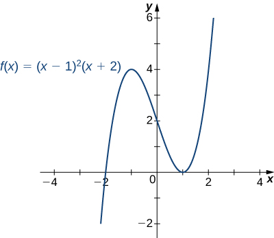
Sketch the graph of
Step 1: The function is defined as long as the denominator is not zero. Therefore, the domain is the set of all real numbers except
Step 2: Find the intercepts. If then so is an intercept. If then which implies Therefore, is the only intercept.
Step 3: Evaluate the limits at infinity. Since is a rational function, divide the numerator and denominator by the highest power in the denominator: We obtain
Therefore, has a horizontal asymptote of as and
Step 4: To determine whether has any vertical asymptotes, first check to see whether the denominator has any zeroes. We find the denominator is zero when To determine whether the lines or are vertical asymptotes of evaluate and By looking at each one-sided limit as we see that
In addition, by looking at each one-sided limit as we find that
Step 5: Calculate the first derivative:
Critical points occur at points where or is undefined. We see that when The derivative is not undefined at any point in the domain of However, are not in the domain of Therefore, to determine where is increasing and where is decreasing, divide the interval into four smaller intervals: and and choose a test point in each interval to determine the sign of in each of these intervals. The values and are good choices for test points as shown in the following table.
| Interval | Test Point | Sign of | Conclusion |
|---|---|---|---|
| is decreasing. | |||
| is decreasing. | |||
| is increasing. | |||
| is increasing. |
From this analysis, we conclude that has a local minimum at but no local maximum.
Step 6: Calculate the second derivative:
To determine the intervals where is concave up and where is concave down, we first need to find all points where or is undefined. Since the numerator for any is never zero. Furthermore, is not undefined for any in the domain of However, as discussed earlier, are not in the domain of Therefore, to determine the concavity of we divide the interval into the three smaller intervals and and choose a test point in each of these intervals to evaluate the sign of in each of these intervals. The values and are possible test points as shown in the following table.
| Interval | Test Point | Sign of | Conclusion |
|---|---|---|---|
| is concave down. | |||
| is concave up. | |||
| is concave down. |
Combining all this information, we arrive at the graph of shown below. Note that, although changes concavity at and there are no inflection points at either of these places because is not continuous at or

Notification Switch
Would you like to follow the 'Calculus volume 1' conversation and receive update notifications?

|
|

|
|

|
|

|
|

|
|
|
|
|

|
|

|
|

|
|

|