

| << Chapter < Page | Chapter >> Page > |
Earlier in this chapter we stated that if a function has a local extremum at a point then must be a critical point of However, a function is not guaranteed to have a local extremum at a critical point. For example, has a critical point at since is zero at but does not have a local extremum at Using the results from the previous section, we are now able to determine whether a critical point of a function actually corresponds to a local extreme value. In this section, we also see how the second derivative provides information about the shape of a graph by describing whether the graph of a function curves upward or curves downward.
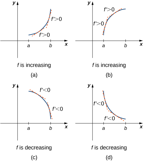
Corollary of the Mean Value Theorem showed that if the derivative of a function is positive over an interval then the function is increasing over On the other hand, if the derivative of the function is negative over an interval then the function is decreasing over as shown in the following figure.
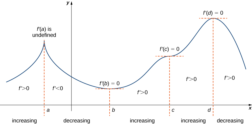
A continuous function has a local maximum at point if and only if switches from increasing to decreasing at point Similarly, has a local minimum at if and only if switches from decreasing to increasing at If is a continuous function over an interval containing and differentiable over except possibly at the only way can switch from increasing to decreasing (or vice versa) at point is if changes sign as increases through If is differentiable at the only way that can change sign as increases through is if Therefore, for a function that is continuous over an interval containing and differentiable over except possibly at the only way can switch from increasing to decreasing (or vice versa) is if or is undefined. Consequently, to locate local extrema for a function we look for points in the domain of such that or is undefined. Recall that such points are called critical points of
Note that need not have a local extrema at a critical point. The critical points are candidates for local extrema only. In [link] , we show that if a continuous function has a local extremum, it must occur at a critical point, but a function may not have a local extremum at a critical point. We show that if has a local extremum at a critical point, then the sign of switches as increases through that point.
Notification Switch
Would you like to follow the 'Calculus volume 1' conversation and receive update notifications?

|
|

|
|
|
|

|
|

|
|

|
|

|
|

|
|

|
|

|