

| << Chapter < Page | Chapter >> Page > |
Find the local linear approximation to at Use it to approximate to five decimal places.
2.00833
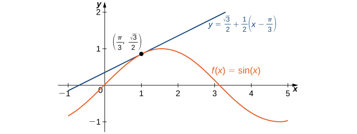
Find the linear approximation of at and use it to approximate
First we note that since rad is equivalent to using the linear approximation at seems reasonable. The linear approximation is given by
We see that
Therefore, the linear approximation of at is given by [link] .
To estimate using we must first convert to radians. We have radians, so the estimate for is given by
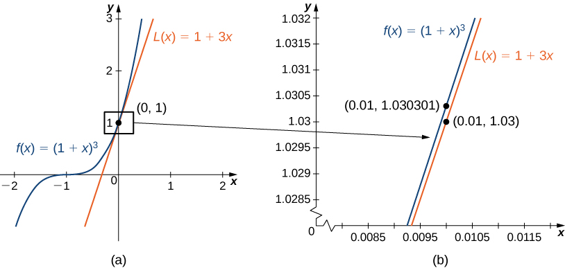
Linear approximations may be used in estimating roots and powers. In the next example, we find the linear approximation for at which can be used to estimate roots and powers for real numbers near 1. The same idea can be extended to a function of the form to estimate roots and powers near a different number
Find the linear approximation of at Use this approximation to estimate
The linear approximation at is given by
Because
the linear approximation is given by [link] (a).
We can approximate by evaluating when We conclude that
Find the linear approximation of at without using the result from the preceding example.
We have seen that linear approximations can be used to estimate function values. They can also be used to estimate the amount a function value changes as a result of a small change in the input. To discuss this more formally, we define a related concept: differentials . Differentials provide us with a way of estimating the amount a function changes as a result of a small change in input values.
When we first looked at derivatives, we used the Leibniz notation to represent the derivative of with respect to Although we used the expressions dy and dx in this notation, they did not have meaning on their own. Here we see a meaning to the expressions dy and dx . Suppose is a differentiable function. Let dx be an independent variable that can be assigned any nonzero real number, and define the dependent variable by
It is important to notice that is a function of both and The expressions dy and dx are called differentials . We can divide both sides of [link] by which yields
This is the familiar expression we have used to denote a derivative. [link] is known as the differential form of [link] .
Notification Switch
Would you like to follow the 'Calculus volume 1' conversation and receive update notifications?

|
|

|
|

|
|

|
|

|
|

|
|
|
|
|

|
|

|
|

|