3.1 Defining the derivative  (Page 4/10)

As the values of $t$ approach $a,$ the values of $v_{\text{ave}}$ approach the value we call the instantaneous velocity    at $a.$ That is, instantaneous velocity at $a,$ denoted $v\left(a\right),$ is given by

To better understand the relationship between average velocity and instantaneous velocity, see [link] . In this figure, the slope of the tangent line (shown in red) is the instantaneous velocity of the object at time $t=a$ whose position at time $t$ is given by the function $s\left(t\right).$ The slope of the secant line (shown in green) is the average velocity of the object over the time interval $\left[a,t\right].$

We can use [link] to calculate the instantaneous velocity, or we can estimate the velocity of a moving object by using a table of values. We can then confirm the estimate by using [link] .

Estimating velocity

A lead weight on a spring is oscillating up and down. Its position at time $t$ with respect to a fixed horizontal line is given by $s\left(t\right)=\text{sin}t$ ( [link] ). Use a table of values to estimate $v\left(0\right).$ Check the estimate by using [link] .

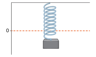
We can estimate the instantaneous velocity at $t=0$ by computing a table of average velocities using values of $t$ approaching $0,$ as shown in [link] .

Average velocities using values of t Approaching 0

$t$	$\frac{\text{sin}t-\text{sin}0}{t-0}=\frac{\text{sin}t}{t}$
$\mathrm{-0.1}$	$0.998334166$
$\mathrm{-0.01}$	$0.9999833333$
$\mathrm{-0.001}$	$0.999999833$
$0.001$	$0.999999833$
$0.01$	$0.9999833333$
$0.1$	$0.998334166$

From the table we see that the average velocity over the time interval $\left[\mathrm{-0.1},0\right]$ is $0.998334166,$ the average velocity over the time interval $\left[\mathrm{-0.01},0\right]$ is $0.9999833333,$ and so forth. Using this table of values, it appears that a good estimate is $v\left(0\right)=1.$

By using [link] , we can see that

$v\left(0\right)=s^{\prime }\left(0\right)=\underset{t\to 0}{\text{lim}}\frac{\text{sin}t-\text{sin}0}{t-0}=\underset{t\to 0}{\text{lim}}\frac{\text{sin}t}{t}=1.$

Thus, in fact, $v\left(0\right)=1.$

Got questions? Get instant answers now!

Got questions? Get instant answers now!

As we have seen throughout this section, the slope of a tangent line to a function and instantaneous velocity are related concepts. Each is calculated by computing a derivative and each measures the instantaneous rate of change of a function, or the rate of change of a function at any point along the function.

Chapter opener: estimating rate of change of velocity

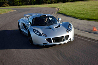
Reaching a top speed of $270.49$ mph, the Hennessey Venom GT is one of the fastest cars in the world. In tests it went from $0$ to $60$ mph in $3.05$ seconds, from $0\text{to}100$ mph in $5.88$ seconds, from $0\text{to}200$ mph in $14.51$ seconds, and from $0\text{to}229.9$ mph in $19.96$ seconds. Use this data to draw a conclusion about the rate of change of velocity (that is, its acceleration ) as it approaches $229.9$ mph. Does the rate at which the car is accelerating appear to be increasing, decreasing, or constant?

First observe that $60$ mph = $88$ ft/s, $100$ mph $\approx 146.67$ ft/s, $200$ mph $\approx 293.33$ ft/s, and $229.9$ mph $\approx 337.19$ ft/s. We can summarize the information in a table.

$v\left(t\right)$ At different values of t

$t$	$v(t)$
$0$	$0$
$3.05$	$88$
$5.88$	$147.67$
$14.51$	$293.33$
$19.96$	$337.19$

Now compute the average acceleration of the car in feet per second on intervals of the form $\left[t,19.96\right]$ as $t$ approaches $19.96,$ as shown in the following table.

Average acceleration

$t$	$\frac{v\left(t\right)-v(19.96)}{t-19.96}=\frac{v\left(t\right)-337.19}{t-19.96}$
$0.0$	$16.89$
$3.05$	$14.74$
$5.88$	$13.46$
$14.51$	$8.05$

The rate at which the car is accelerating is decreasing as its velocity approaches $229.9$ mph $\text{(}337.19$ ft/s).

Got questions? Get instant answers now!

Got questions? Get instant answers now!