

| << Chapter < Page | Chapter >> Page > |
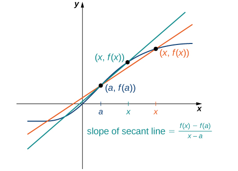
The secant to the function through the points and is the line passing through these points. Its slope is given by
The accuracy of approximating the rate of change of the function with a secant line depends on how close x is to a . As we see in [link] , if x is closer to a , the slope of the secant line is a better measure of the rate of change of at a .
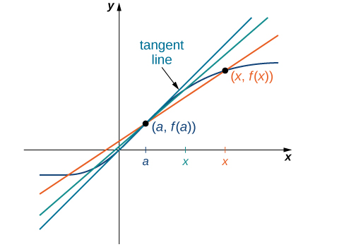
The secant lines themselves approach a line that is called the tangent to the function at a ( [link] ). The slope of the tangent line to the graph at a measures the rate of change of the function at a . This value also represents the derivative of the function at a , or the rate of change of the function at a . This derivative is denoted by Differential calculus is the field of calculus concerned with the study of derivatives and their applications.
For an interactive demonstration of the slope of a secant line that you can manipulate yourself, visit this applet ( Note: this site requires a Java browser plugin): Math Insight .
[link] illustrates how to find slopes of secant lines. These slopes estimate the slope of the tangent line or, equivalently, the rate of change of the function at the point at which the slopes are calculated.
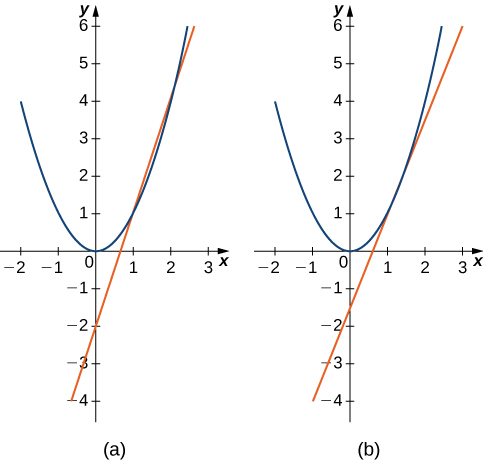
Estimate the slope of the tangent line (rate of change) to at by finding slopes of secant lines through and each of the following points on the graph of
Use the formula for the slope of a secant line from the definition.
The point in part b. is closer to the point so the slope of 2.5 is closer to the slope of the tangent line. A good estimate for the slope of the tangent would be in the range of 2 to 2.5 ( [link] ).
Estimate the slope of the tangent line (rate of change) to at by finding slopes of secant lines through and the point on the graph of
2.25
We continue our investigation by exploring a related question. Keeping in mind that velocity may be thought of as the rate of change of position, suppose that we have a function, that gives the position of an object along a coordinate axis at any given time t . Can we use these same ideas to create a reasonable definition of the instantaneous velocity at a given time We start by approximating the instantaneous velocity with an average velocity. First, recall that the speed of an object traveling at a constant rate is the ratio of the distance traveled to the length of time it has traveled. We define the average velocity of an object over a time period to be the change in its position divided by the length of the time period.
Notification Switch
Would you like to follow the 'Calculus volume 1' conversation and receive update notifications?

|
|

|
|

|
|

|
|

|
|

|
|

|
|

|
|

|
|
|
|