<< Chapter < Page Chapter >> Page >

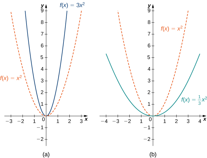
A vertical scaling of a graph occurs if we multiply all outputs y of a function by the same positive constant. For c > 0 , the graph of the function c f ( x ) is the graph of f ( x ) scaled vertically by a factor of c . If c > 1 , the values of the outputs for the function c f ( x ) are larger than the values of the outputs for the function f ( x ) ; therefore, the graph has been stretched vertically. If 0 < c < 1 , then the outputs of the function c f ( x ) are smaller, so the graph has been compressed. For example, the graph of the function f ( x ) = 3 x 2 is the graph of y = x 2 stretched vertically by a factor of 3, whereas the graph of f ( x ) = x 2 / 3 is the graph of y = x 2 compressed vertically by a factor of 3 ( [link] ).

An image of two graphs. The first graph is labeled “a” and has an x axis that runs from -3 to 3 and a y axis that runs from -2 to 9. The graph is of two functions. The first function is “f(x) = x squared”, which is a parabola that decreases until the origin and then increases again after the origin. The second function is “f(x) = 3(x squared)”, which is a parabola that decreases until the origin and then increases again after the origin, but is vertically stretched and thus increases at a quicker rate than the first function. The second graph is labeled “b” and has an x axis that runs from -4 to 4 and a y axis that runs from -2 to 9. The graph is of two functions. The first function is “f(x) = x squared”, which is a parabola that decreases until the origin and then increases again after the origin. The second function is “f(x) = (1/3)(x squared)”, which is a parabola that decreases until the origin and then increases again after the origin, but is vertically compressed and thus increases at a slower rate than the first function.
(a) If c > 1 , the graph of y = c f ( x ) is a vertical stretch of the graph of y = f ( x ) . (b) If 0 < c < 1 , the graph of y = c f ( x ) is a vertical compression of the graph of y = f ( x ) .

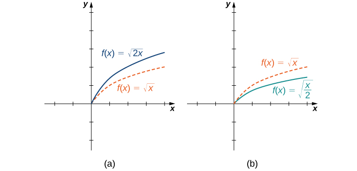
The horizontal scaling of a function occurs if we multiply the inputs x by the same positive constant. For c > 0 , the graph of the function f ( c x ) is the graph of f ( x ) scaled horizontally by a factor of c . If c > 1 , the graph of f ( c x ) is the graph of f ( x ) compressed horizontally. If 0 < c < 1 , the graph of f ( c x ) is the graph of f ( x ) stretched horizontally. For example, consider the function f ( x ) = 2 x and evaluate f at x / 2 . Since f ( x / 2 ) = x , the graph of f ( x ) = 2 x is the graph of y = x compressed horizontally. The graph of y = x / 2 is a horizontal stretch of the graph of y = x ( [link] ).

An image of two graphs. Both graphs have an x axis that runs from -2 to 4 and a y axis that runs from -2 to 5. The first graph is labeled “a” and is of two functions. The first graph is of two functions. The first function is “f(x) = square root of x”, which is a curved function that begins at the origin and increases. The second function is “f(x) = square root of 2x”, which is a curved function that begins at the origin and increases, but increases at a faster rate than the first function. The second graph is labeled “b” and is of two functions. The first function is “f(x) = square root of x”, which is a curved function that begins at the origin and increases. The second function is “f(x) = square root of (x/2)”, which is a curved function that begins at the origin and increases, but increases at a slower rate than the first function.
(a) If c > 1 , the graph of y = f ( c x ) is a horizontal compression of the graph of y = f ( x ) . (b) If 0 < c < 1 , the graph of y = f ( c x ) is a horizontal stretch of the graph of y = f ( x ) .

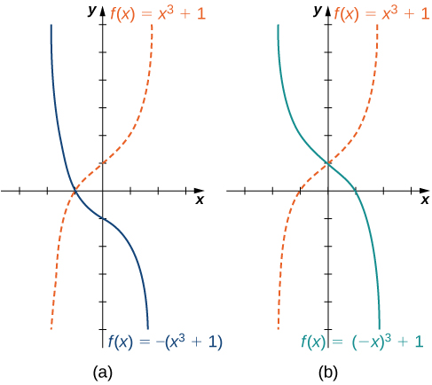
We have explored what happens to the graph of a function f when we multiply f by a constant c > 0 to get a new function c f ( x ) . We have also discussed what happens to the graph of a function f when we multiply the independent variable x by c > 0 to get a new function f ( c x ) . However, we have not addressed what happens to the graph of the function if the constant c is negative. If we have a constant c < 0 , we can write c as a positive number multiplied by −1 ; but, what kind of transformation do we get when we multiply the function or its argument by −1 ? When we multiply all the outputs by −1 , we get a reflection about the x -axis. When we multiply all inputs by −1 , we get a reflection about the y -axis. For example, the graph of f ( x ) = ( x 3 + 1 ) is the graph of y = ( x 3 + 1 ) reflected about the x -axis. The graph of f ( x ) = ( x ) 3 + 1 is the graph of y = x 3 + 1 reflected about the y -axis ( [link] ).

An image of two graphs. Both graphs have an x axis that runs from -3 to 3 and a y axis that runs from -5 to 6. The first graph is labeled “a” and is of two functions. The first graph is of two functions. The first function is “f(x) = x cubed + 1”, which is a curved increasing function that has an x intercept at (-1, 0) and a y intercept at (0, 1). The second function is “f(x) = -(x cubed + 1)”, which is a curved decreasing function that has an x intercept at (-1, 0) and a y intercept at (0, -1). The second graph is labeled “b” and is of two functions. The first function is “f(x) = x cubed + 1”, which is a curved increasing function that has an x intercept at (-1, 0) and a y intercept at (0, 1). The second function is “f(x) = (-x) cubed + 1”, which is a curved decreasing function that has an x intercept at (1, 0) and a y intercept at (0, 1). The first function increases at the same rate the second function decreases for the same values of x.
(a) The graph of y = f ( x ) is the graph of y = f ( x ) reflected about the x -axis. (b) The graph of y = f ( x ) is the graph of y = f ( x ) reflected about the
y -axis.

If the graph of a function consists of more than one transformation of another graph, it is important to transform the graph in the correct order. Given a function f ( x ) , the graph of the related function y = c f ( a ( x + b ) ) + d can be obtained from the graph of y = f ( x ) by performing the transformations in the following order.

  1. Horizontal shift of the graph of y = f ( x ) . If b > 0 , shift left. If b < 0 , shift right.
  2. Horizontal scaling of the graph of y = f ( x + b ) by a factor of | a | . If a < 0 , reflect the graph about the y -axis.
  3. Vertical scaling of the graph of y = f ( a ( x + b ) ) by a factor of | c | . If c < 0 , reflect the graph about the x -axis.
  4. Vertical shift of the graph of y = c f ( a ( x + b ) ) . If d > 0 , shift up. If d < 0 , shift down.

Get Jobilize Job Search Mobile App in your pocket Now!

Get it on Google Play Download on the App Store Now


Source:  OpenStax, Calculus volume 1. OpenStax CNX. Feb 05, 2016 Download for free at http://cnx.org/content/col11964/1.2
Google Play and the Google Play logo are trademarks of Google Inc.

Notification Switch

Would you like to follow the 'Calculus volume 1' conversation and receive update notifications?

Ask