<< Chapter < Page Chapter >> Page >
 Photo (a) shows penguins, which maintain a defined territory and, therefore, have a uniform distribution. Photo (b) shows a field of dandelions whose seeds are dispersed by wind, resulting in a random distribution patter. Photo (c) shows elephants, which travel in herds resulting in a clumped distribution pattern.
Species may have a random, clumped, or uniform distribution. Plants such as (a) dandelions with wind-dispersed seeds tend to be randomly distributed. Animals such as (b) elephants that travel in groups exhibit a clumped distribution. Territorial birds such as (c) penguins tend to have a uniform distribution. (credit a: modification of work by Rosendahl; credit b: modification of work by Rebecca Wood; credit c: modification of work by Ben Tubby)

Demography

While population size and density describe a population at one particular point in time, scientists must use demography to study the dynamics of a population. Demography is the statistical study of population changes over time: birth rates, death rates, and life expectancies. These population characteristics are often displayed in a life table.

Life tables

Life tables provide important information about the life history of an organism and the life expectancy of individuals at each age. They are modeled after actuarial tables used by the insurance industry for estimating human life expectancy. Life tables may include the probability of each age group dying before their next birthday, the percentage of surviving individuals dying at a particular age interval (their mortality rate    , and their life expectancy at each interval. An example of a life table is shown in [link] from a study of Dall mountain sheep, a species native to northwestern North America. Notice that the population is divided into age intervals (column A). The mortality rate (per 1000) shown in column D is based on the number of individuals dying during the age interval (column B), divided by the number of individuals surviving at the beginning of the interval (Column C) multiplied by 1000.

mortality rate  =   number of individuals dying number of individuals surviving   ×   1000

For example, between ages three and four, 12 individuals die out of the 776 that were remaining from the original 1000 sheep. This number is then multiplied by 1000 to give the mortality rate per thousand.

mortality rate  =   12 776   ×   1000     15.5

As can be seen from the mortality rate data (column D), a high death rate occurred when the sheep were between six months and a year old, and then increased even more from 8 to 12 years old, after which there were few survivors. The data indicate that if a sheep in this population were to survive to age one, it could be expected to live another 7.7 years on average, as shown by the life-expectancy numbers in column E.

This life table of Ovis dalli shows the number of deaths, number of survivors, mortality rate, and life expectancy at each age interval for Dall mountain sheep.
Life Table of Dall Mountain Sheep Data Adapted from Edward S. Deevey, Jr., “Life Tables for Natural Populations of Animals,” The Quarterly Review of Biology 22, no. 4 (December 1947): 283-314.
A B C D E
Age interval (years) Number dying in age interval out of 1000 born Number surviving at beginning of age interval out of 1000 born Mortality rate per 1000 alive at beginning of age interval Life expectancy or mean lifetime remaining to those attaining age interval
0–0.5 54 1000 54.0 7.06
0.5–1 145 946 153.3
1–2 12 801 15.0 7.7
2–3 13 789 16.5 6.8
3–4 12 776 15.5 5.9
4–5 30 764 39.3 5.0
5–6 46 734 62.7 4.2
6–7 48 688 69.8 3.4
7–8 69 640 107.8 2.6
8–9 132 571 231.2 1.9
9–10 187 439 426.0 1.3
10–11 156 252 619.0 0.9
11–12 90 96 937.5 0.6
12–13 3 6 500.0 1.2
13–14 3 3 1000 0.7

Survivorship curves

Another tool used by population ecologists is a survivorship curve    , which is a graph of the number of individuals surviving at each age interval versus time. These curves allow us to compare the life histories of different populations ( [link] ). There are three types of survivorship curves. In a type I curve, mortality is low in the early and middle years and occurs mostly in older individuals. Organisms exhibiting a type I survivorship typically produce few offspring and provide good care to the offspring increasing the likelihood of their survival. Humans and most mammals exhibit a type I survivorship curve. In type II curves, mortality is relatively constant throughout the entire life span, and mortality is equally likely to occur at any point in the life span. Many bird populations provide examples of an intermediate or type II survivorship curve. In type III survivorship curves, early ages experience the highest mortality with much lower mortality rates for organisms that make it to advanced years. Type III organisms typically produce large numbers of offspring, but provide very little or no care for them. Trees and marine invertebrates exhibit a type III survivorship curve because very few of these organisms survive their younger years, but those that do make it to an old age are more likely to survive for a relatively long period of time.

 Graph plots the log of number of individuals surviving versus time. Three curves are shown, representing type I, type II, and type III survivorship patterns. Birds exhibit a type II survivorship curve, which decreases linearly with time. Humans show a type I survivorship curve, which starts with a gentle slope that becomes increasingly steep with time. Trees show a type III survivorship pattern, which starts with a steep slope that becomes less steep with time.
Survivorship curves show the distribution of individuals in a population according to age. Humans and most mammals have a Type I survivorship curve, because death primarily occurs in the older years. Birds have a Type II survivorship curve, as death at any age is equally probable. Trees have a Type III survivorship curve because very few survive the younger years, but after a certain age, individuals are much more likely to survive.

Section summary

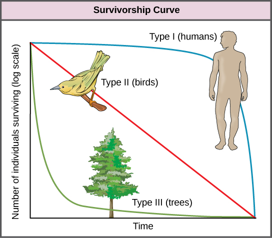
Populations are individuals of a species that live in a particular habitat. Ecologists measure characteristics of populations: size, density, and distribution pattern. Life tables are useful to calculate life expectancies of individual population members. Survivorship curves show the number of individuals surviving at each age interval plotted versus time.

[link] As this graph shows, population density typically decreases with increasing body size. Why do you think this is the case?

[link] Smaller animals require less food and others resources, so the environment can support more of them per unit area.

Got questions? Get instant answers now!

Questions & Answers

What are the factors that affect demand for a commodity
Florence Reply
differentiate between demand and supply giving examples
Lambiv Reply
differentiated between demand and supply using examples
Lambiv
what is labour ?
Lambiv
how will I do?
Venny Reply
how is the graph works?I don't fully understand
Rezat Reply
information
Eliyee
devaluation
Eliyee
t
WARKISA
hi guys good evening to all
Lambiv
multiple choice question
Aster Reply
appreciation
Eliyee
explain perfect market
Lindiwe Reply
In economics, a perfect market refers to a theoretical construct where all participants have perfect information, goods are homogenous, there are no barriers to entry or exit, and prices are determined solely by supply and demand. It's an idealized model used for analysis,
Ezea
What is ceteris paribus?
Shukri Reply
other things being equal
AI-Robot
When MP₁ becomes negative, TP start to decline. Extuples Suppose that the short-run production function of certain cut-flower firm is given by: Q=4KL-0.6K2 - 0.112 • Where is quantity of cut flower produced, I is labour input and K is fixed capital input (K-5). Determine the average product of lab
Kelo
Extuples Suppose that the short-run production function of certain cut-flower firm is given by: Q=4KL-0.6K2 - 0.112 • Where is quantity of cut flower produced, I is labour input and K is fixed capital input (K-5). Determine the average product of labour (APL) and marginal product of labour (MPL)
Kelo
yes,thank you
Shukri
Can I ask you other question?
Shukri
what is monopoly mean?
Habtamu Reply
What is different between quantity demand and demand?
Shukri Reply
Quantity demanded refers to the specific amount of a good or service that consumers are willing and able to purchase at a give price and within a specific time period. Demand, on the other hand, is a broader concept that encompasses the entire relationship between price and quantity demanded
Ezea
ok
Shukri
how do you save a country economic situation when it's falling apart
Lilia Reply
what is the difference between economic growth and development
Fiker Reply
Economic growth as an increase in the production and consumption of goods and services within an economy.but Economic development as a broader concept that encompasses not only economic growth but also social & human well being.
Shukri
production function means
Jabir
What do you think is more important to focus on when considering inequality ?
Abdisa Reply
any question about economics?
Awais Reply
sir...I just want to ask one question... Define the term contract curve? if you are free please help me to find this answer 🙏
Asui
it is a curve that we get after connecting the pareto optimal combinations of two consumers after their mutually beneficial trade offs
Awais
thank you so much 👍 sir
Asui
In economics, the contract curve refers to the set of points in an Edgeworth box diagram where both parties involved in a trade cannot be made better off without making one of them worse off. It represents the Pareto efficient allocations of goods between two individuals or entities, where neither p
Cornelius
In economics, the contract curve refers to the set of points in an Edgeworth box diagram where both parties involved in a trade cannot be made better off without making one of them worse off. It represents the Pareto efficient allocations of goods between two individuals or entities,
Cornelius
Suppose a consumer consuming two commodities X and Y has The following utility function u=X0.4 Y0.6. If the price of the X and Y are 2 and 3 respectively and income Constraint is birr 50. A,Calculate quantities of x and y which maximize utility. B,Calculate value of Lagrange multiplier. C,Calculate quantities of X and Y consumed with a given price. D,alculate optimum level of output .
Feyisa Reply
Answer
Feyisa
c
Jabir
the market for lemon has 10 potential consumers, each having an individual demand curve p=101-10Qi, where p is price in dollar's per cup and Qi is the number of cups demanded per week by the i th consumer.Find the market demand curve using algebra. Draw an individual demand curve and the market dema
Gsbwnw Reply
suppose the production function is given by ( L, K)=L¼K¾.assuming capital is fixed find APL and MPL. consider the following short run production function:Q=6L²-0.4L³ a) find the value of L that maximizes output b)find the value of L that maximizes marginal product
Abdureman
Got questions? Join the online conversation and get instant answers!
Jobilize.com Reply

Get Jobilize Job Search Mobile App in your pocket Now!

Get it on Google Play Download on the App Store Now


Source:  OpenStax, Concepts of biology. OpenStax CNX. Feb 29, 2016 Download for free at http://cnx.org/content/col11487/1.9
Google Play and the Google Play logo are trademarks of Google Inc.

Notification Switch

Would you like to follow the 'Concepts of biology' conversation and receive update notifications?

Ask