

| << Chapter < Page | Chapter >> Page > |
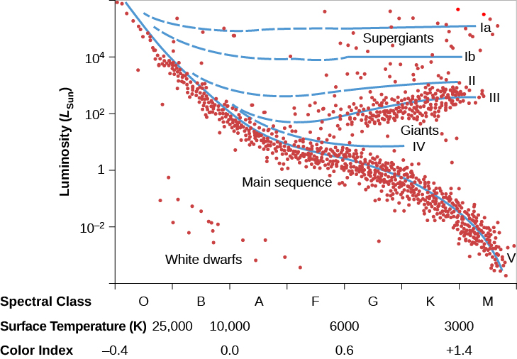
With both its spectral and luminosity classes known, a star’s position on the H–R diagram is uniquely determined. Since the diagram plots luminosity versus temperature, this means we can now read off the star’s luminosity (once its spectrum has helped us place it on the diagram). As before, if we know how luminous the star really is and see how dim it looks, the difference allows us to calculate its distance. (For historical reasons, astronomers sometimes call this method of distance determination spectroscopic parallax , even though the method has nothing to do with parallax.)
The H–R diagram method allows astronomers to estimate distances to nearby stars, as well as some of the most distant stars in our Galaxy, but it is anchored by measurements of parallax. The distances measured using parallax are the gold standard for distances: they rely on no assumptions, only geometry. Once astronomers take a spectrum of a nearby star for which we also know the parallax, we know the luminosity that corresponds to that spectral type. Nearby stars thus serve as benchmarks for more distant stars because we can assume that two stars with identical spectra have the same intrinsic luminosity.
Introductory textbooks such as ours work hard to present the material in a straightforward and simplified way. In doing so, we sometimes do our students a disservice by making scientific techniques seem too clean and painless. In the real world, the techniques we have just described turn out to be messy and difficult, and often give astronomers headaches that last long into the day.
For example, the relationships we have described such as the period-luminosity relation for certain variable stars aren’t exactly straight lines on a graph. The points representing many stars scatter widely when plotted, and thus, the distances derived from them also have a certain built-in scatter or uncertainty.
The distances we measure with the methods we have discussed are therefore only accurate to within a certain percentage of error—sometimes 10%, sometimes 25%, sometimes as much as 50% or more. A 25% error for a star estimated to be 10,000 light-years away means it could be anywhere from 7500 to 12,500 light-years away. This would be an unacceptable uncertainty if you were loading fuel into a spaceship for a trip to the star, but it is not a bad first figure to work with if you are an astronomer stuck on planet Earth.
Nor is the construction of H–R diagrams as easy as you might think at first. To make a good diagram, one needs to measure the characteristics and distances of many stars, which can be a time-consuming task. Since our own solar neighborhood is already well mapped, the stars astronomers most want to study to advance our knowledge are likely to be far away and faint. It may take hours of observing to obtain a single spectrum. Observers may have to spend many nights at the telescope (and many days back home working with their data) before they get their distance measurement. Fortunately, this is changing because surveys like Gaia will study billions of stars, producing public datasets that all astronomers can use.
Notification Switch
Would you like to follow the 'Astronomy' conversation and receive update notifications?

|
|

|
|

|
|

|
|

|
|

|
|
|
|
|

|
|
|
|
|

|